Monolayer MoS2 example: building a minimal Wannier tight-binding model
- 0. How do we choose the orbital projections?
- 1. Generate the k-mesh
- 2. Run the self-consistent DFT calculation
- 3. Calculate the DFT band structure
- 4. Run the SCF calculation again before Wannier90
- 5. Prepare the Wannier90 input file
- 6. Choose the orbital projections
- 7. Define the frozen energy window
- 8. Define the outer disentanglement window
- 9. Run Wannier90 preprocessing
- 10. Run pw2wannier90.x
- 11. Run Wannier90
- 12. How to check that the Wannier90 calculation is converged
- 13. Plot the band structure
- What should we learn from this example?
In this example, we will build a simple tight-binding model for monolayer MoS2 using Wannier90. Our goal is to reproduce the most important low-energy electronic bands: the valence-band maximum (VBM), the conduction-band minimum (CBM), and the next conduction band (CBM+1).
The important point is that we will describe these three bands using only three Wannier functions. This is one of the most powerful ideas behind Wannier90: instead of working with many complicated Bloch wave functions from DFT, we construct a compact real-space model that keeps only the essential physics.
For monolayer MoS2, a very good minimal model can be built from three molybdenum d-orbitals:
Mo:dz2
Mo:dxy
Mo:dx2-y2
These orbitals are physically meaningful because the band edges of MoS2 near the gap are dominated mainly by Mo d-states. Therefore, this three-orbital model is not just a numerical trick — it has a clear chemical and physical interpretation.
You can download the required input files for this example here.
0. How do we choose the orbital projections?
Before choosing the Wannier projections, we need to understand the orbital character of the bands that we want to reproduce.
In this tutorial, our goal is to build a minimal three-band model for monolayer MoS2. We want to describe the three most important bands near the band gap:
$$\text{VBM}, \quad \text{CBM}, \quad \text{CBM+1}$$
The natural question is:
Why can these three bands be described by three Mo d-orbitals?The answer comes from the electronic structure of monolayer MoS2. Near the band gap, the relevant states are mainly formed by molybdenum d-orbitals. In particular, a very good minimal basis is:
Mo:dz2
Mo:dxy
Mo:dx2-y2
These orbitals are especially important because the band-edge states in MoS2 are dominated by Mo d-states rather than sulfur p-states.
Physically, this means that the low-energy electronic motion near the gap mostly takes place on the Mo atoms. Sulfur atoms are still very important for the full crystal structure and bonding, but for a minimal low-energy model around the band gap, the dominant orbital contribution comes from these three Mo d-orbitals.
0.1 Why these particular three orbitals?
Molybdenum has five d-orbitals:
$$d_{z^2}, \quad d_{xy}, \quad d_{x^2-y^2}, \quad d_{xz}, \quad d_{yz}$$
However, not all of them contribute equally to the electronic states near the band gap, particularly the valence- and conduction-band edges of monolayer MoS2.
For the usual low-energy model near the gap, the most important orbitals are:
$$d_{z^2}, \quad d_{xy}, \quad d_{x^2-y^2}$$
The $d_{z^2}$ orbital strongly contributes to the conduction-band minimum near the K point. The $d_{xy}$ and $d_{x^2-y^2}$ orbitals strongly contribute to the valence-band maximum and to the nearby conduction bands.
Therefore, if we want a compact model for VBM, CBM, and CBM+1, these three orbitals are a very natural choice.
This is why we use the following projections in Wannier90:
begin projections
Mo:dz2
Mo:dxy
Mo:dx2-y2
end projections
The number of projections is equal to the number of Wannier functions:
3 projections → 3 Wannier functions → 3-band tight-binding modelThis gives a minimal and physically transparent model. More detailed explanation.
0.2 How can students find which orbitals to use?
There are several practical ways to choose projections.
The first and most important method is to look at the orbital-projected band structure or projected density of states.
In Quantum ESPRESSO, this can be done using tools such as:
projwfc.xThis program projects the DFT wave functions onto atomic orbitals and shows which atoms and orbitals contribute to each band.
After running a projected analysis, students can answer questions such as:
- Is this band mostly Mo d?
- Is it mostly S p?
- Which d-orbitals are important?
- Do the target bands have the same orbital character along the whole k-path?
For monolayer MoS2, this analysis shows that the bands near the gap are mainly Mo d-like. This is why Mo d-orbital projections are a good starting point.
0.3 Can we choose projections directly from the band structure?
The ordinary band structure alone shows the band energies, but it does not directly show the orbital character. From the band structure, we can see which bands we want to reproduce, but we cannot reliably know which atomic orbitals form these bands.
Therefore, the band structure answers the question:
Which bands do we want?but the projected band structure or projected density of states answers the question:
Which orbitals form these bands?For Wannier90, we need both pieces of information.
First, we identify the energy range and target bands from the band structure. Then, we use orbital projections, projected density of states, or literature information to determine the orbital character of these bands.
0.4 Practical strategy for choosing Wannier projections
A good practical strategy is:
- Calculate the DFT band structure.
- Identify the bands that you want to reproduce.
- Calculate orbital projections or projected density of states.
- Find which atoms and orbitals dominate the target bands.
- Use these orbitals as initial projections in Wannier90.
- Check whether the Wannier-interpolated bands reproduce the DFT bands.
For example, in monolayer MoS2:
Target bands:
VBM, CBM, CBM+1

Dominant orbital character:
Mo d-states

Minimal Wannier projections:
Mo:dz2
Mo:dxy
Mo:dx2-y2
This gives a compact three-band model.
0.5 What if the Wannier model is not good?
The first choice of projections is not always perfect. If the Wannier-interpolated bands do not reproduce the DFT bands well, this may mean that the chosen orbital basis is incomplete.
For example, one may need to include additional orbitals:
Mo:dxz
Mo:dyz
S:px
S:py
S:pz
This would increase the number of Wannier functions and produce a larger tight-binding model.
A larger model is usually less minimal, but it may be more accurate over a wider energy range.
This is a general trade-off in Wannier90:
Small number of Wannier functions:
simple, elegant, easy to interpret, but valid only in a limited energy range.

Larger number of Wannier functions:
more accurate over a wider energy range, but less compact and less intuitive.
In this tutorial, we intentionally choose the minimal three-band model because it is simple and clearly demonstrates the main idea of Wannierization.
0.6 The main lesson
The choice of projections is not arbitrary. It is based on the orbital character of the bands.
For monolayer MoS2, the bands near the gap are mainly formed by Mo d-orbitals. Therefore, the projections
Mo:dz2
Mo:dxy
Mo:dx2-y2
are physically motivated and lead to a compact three-band model for VBM, CBM, and CBM+1.
In general, students should not guess projections blindly. They should first inspect the band structure, projected density of states, orbital-projected bands, or reliable literature, and then choose projections that match the physical character of the target bands.
1. Generate the k-mesh
First, we generate a uniform k-point mesh using the kmesh.pl utility from the Wannier90/utility/ folder:
kmesh.pl 15 15 1
This command generates a $15 \times 15 \times 1$ k-mesh. Since monolayer MoS2 is a two-dimensional system, we use only one k-point in the out-of-plane direction.
The generated k-points should be inserted into the scf.in input file for Quantum ESPRESSO.
2. Run the self-consistent DFT calculation
Now we run the self-consistent field calculation with Quantum ESPRESSO:
pw.x < scf.in > scf.out
This step calculates the ground-state charge density of the system. In simple words, QE first needs to determine how electrons are distributed in the material before we can calculate band structures or construct Wannier functions.
This calculation is the foundation for all later steps.
3. Calculate the DFT band structure
After the SCF calculation, we calculate the band structure using QE:
pw.x < bands.in > bands.out
bands.x < bandsx.in > bandsx.out
In bands.in, we use the automatic generation of high-symmetry k-points along the path
$$\Gamma \rightarrow M \rightarrow K \rightarrow \Gamma$$
The corresponding block is:
K_POINTS crystal_b
4
gG   10
M    10
K    10
gG   10
Here, 4 means that we define four high-symmetry points. The number 10 after each point means that QE will generate 10 intermediate points between this point and the next one.
This DFT band structure will later serve as our reference. The Wannier-interpolated bands must reproduce it well in the energy region of interest. This comparison is one of the most important checks that the Wannier model is correct.
4. Run the SCF calculation again before Wannier90
Before running Wannier90, we need to run the QE SCF calculation again:
pw.x < scf.in > scf.out
This is necessary because the band-structure calculation can overwrite or modify some QE data files needed by pw2wannier90.x.
To avoid repeating the full SCF cycle from scratch, we can restart from the previously calculated charge density by adding:
&electrons
    startingpot = 'file'
/
This tells QE to read the previous potential from file, which usually makes the calculation faster.
5. Prepare the Wannier90 input file
The Wannier90 input file is d.win.
There are two very important ingredients that must be consistent with the QE calculation:
- the uniform k-mesh;
- the high-symmetry k-path for plotting the band structure.
The same k-mesh generated by kmesh.pl and used in scf.in must also be inserted into d.win.
For the band-structure path, it is best to use the exact k-path generated by QE. We extract it from the QE output in reciprocal crystal coordinates and insert it into d.win:
begin kpoint_path
G 0.0       0.0      0.0
M 0.5       0.0      0.0
M 0.5       0.0      0.0
K 0.666667 -0.333333 0.0
K 0.666667 -0.333333 0.0
G 0.0       0.0      0.0
end kpoint_path
This is a small but important technical detail. If the Wannier90 path is not the same as the QE path, the comparison between QE bands and Wannier-interpolated bands may look confusing or even incorrect.
6. Choose the orbital projections
For the minimal three-band model of MoS2, we use three Mo d-orbitals:
begin projections
Mo:dz2
Mo:dxy
Mo:dx2-y2
end projections
These projections are the initial guess for Wannier90. They tell the program what kind of localized orbitals we expect.
This step is very important conceptually. Wannier90 does not blindly create arbitrary localized functions. Instead, we guide it by saying:
“We expect the relevant low-energy bands to come mainly from these Mo d-orbitals.”
If the choice of projections is physically reasonable, the resulting Wannier functions are usually better localized, and the Wannier-interpolated band structure is more accurate.
7. Define the frozen energy window
We want to construct exactly three Wannier functions. Therefore, we need to select an energy range where only the three target bands are present.
This is done using the frozen window:
dis_froz_min  = -1.90
dis_froz_max  =  1.53
The frozen window tells Wannier90:
“These bands must be reproduced exactly as part of the target subspace.”
In this example, the frozen window is chosen so that it contains only the three bands of interest: VBM, CBM, and CBM+1.
If Wannier90 finds more than three bands inside the frozen window at any k-point, it will stop with an error message. This is not necessarily a bad thing. It simply means that the frozen window is too wide and must be narrowed.
This is one of the most common practical issues when learning Wannier90. The number of bands inside the frozen window must be compatible with the number of Wannier functions.
8. Define the outer disentanglement window
In addition to the frozen window, we also define a wider outer energy window:
dis_win_min   = -5.0
dis_win_max   =  4.5
This window is used during the disentanglement procedure. What is disentanglement?
The idea is the following. In real materials, the bands we want are often mixed with other bands. Wannier90 therefore needs some freedom to search for the best three-dimensional subspace inside a larger energy range.
The frozen window says: “These bands are mandatory.”
The outer window says: “Search for the best Wannier subspace inside this larger energy region.”
This distinction is essential. The frozen window protects the bands we definitely want, while the outer window gives Wannier90 enough flexibility to construct smooth and localized Wannier functions.
9. Run Wannier90 preprocessing
Before running the QE-to-Wannier interface, we first run Wannier90 in preprocessing mode:
wannier90.x -pp d
This command reads the input file:
d.win
and generates auxiliary files needed by pw2wannier90.x.
The name d is the seedname. Therefore, Wannier90 expects the input file to be called:
d.win
10. Run pw2wannier90.x
Now we run the interface between Quantum ESPRESSO and Wannier90:
pw2wannier90.x -in pw2wan.in
This step calculates the overlap matrices and projection matrices needed by Wannier90.
In simple terms, pw2wannier90.x transfers the information from the plane-wave DFT calculation into the format required for constructing Wannier functions.
This is the bridge between QE and Wannier90.
11. Run Wannier90
Now we run Wannier90:
wannier90.x d
This command again uses the same input file:
d.win
At this stage, Wannier90 performs the disentanglement and localization procedures, constructs the Wannier functions, and calculates the Wannier-interpolated band structure.
This is the central step of the whole workflow.
12. How to check that the Wannier90 calculation is converged
Running Wannier90 is not the end of the calculation. After the command
wannier90.x dwe must check whether the obtained Wannier functions are physically meaningful and whether the Wannier-interpolated bands reproduce the original DFT bands.
This is a very important step. Wannier90 can finish without errors, but the resulting tight-binding model may still be poor if the projections, energy windows, or convergence parameters were not chosen well.
In practice, we should check several things.
12.1 Check the band interpolation
The most important test is the comparison between the original QE band structure and the Wannier-interpolated band structure.
If the Wannier model is good, the Wannier-interpolated bands should closely follow the QE bands in the target energy region. In this example, the target bands are:
- VBM,
- CBM,
- CBM+1.
The agreement does not need to be perfect for all high-energy bands. What matters is that the three bands of interest are accurately reproduced.
If the Wannier bands do not match the QE bands, possible reasons are:
- the initial orbital projections are not appropriate;
- the frozen energy window is too wide or too narrow;
- the outer disentanglement window is poorly chosen;
- the number of Wannier functions is too small;
- the disentanglement procedure did not converge well;
- the k-mesh is too coarse.
For this MoS2 example, a good result means that the three-band Wannier model reproduces the DFT bands near the band gap along the path
$$\Gamma \rightarrow M \rightarrow K \rightarrow \Gamma$$
This comparison is usually the first and most important quality check.
12.2 Check the spread convergence
Wannier90 minimizes the spatial spread of the Wannier functions. During the calculation, it prints the spread values into the main output file:
d.woutThe spread describes how localized the Wannier functions are in real space. In simple words, smaller spread usually means more localized Wannier functions.
In the output file, one should look for the final spread:
Final Stateand the total spread:
Omega Totalor similar lines printed near the end of the file.
A successful calculation usually shows that the spread decreases during the iterations and then becomes stable. This means that the localization procedure has converged.
If the spread still changes strongly at the end of the calculation, it may mean that the number of iterations is not enough.
The number of localization iterations is controlled by the parameter:
num_iterFor example:
num_iter = 1000For simple systems, a few hundred iterations may already be enough. For more complicated systems, especially when disentanglement is used, it is common to use 1000 or even several thousand iterations.
There is no universal “magic number.” The important thing is not the number of iterations itself, but whether the spread has stopped changing significantly.
A practical rule is:
If increasing num_iter does not change the final spread and the band structure,
then the localization procedure is converged.
12.3 Check disentanglement convergence
When the number of DFT bands inside the outer energy window is larger than the number of Wannier functions, Wannier90 performs disentanglement. In this example, we construct only three Wannier functions, but the outer window contains more than three DFT bands.
The disentanglement procedure is controlled by parameters such as:
dis_num_iterFor example:
dis_num_iter = 1000The disentanglement step tries to find a smooth three-dimensional band subspace from the larger set of DFT bands.
This step is especially important when target bands are close to other bands or mixed with them.
To check convergence, open:
d.woutand inspect the disentanglement section. The relevant quantity should become stable during iterations. If the disentanglement has not converged, the final Wannier bands may look irregular or may not reproduce the QE bands well.
Typical values are:
dis_num_iter = 500or
dis_num_iter = 1000For more difficult cases, one can increase it further:
dis_num_iter = 2000Again, the best criterion is practical: after increasing dis_num_iter, the final bands and spreads should no longer change.
12.4 Check the Wannier centers
Another very useful check is to inspect the positions of the Wannier centers.
Wannier centers are printed in the output file:
d.woutNear the end of the file, Wannier90 prints a block with the final centers and spreads of the Wannier functions. It usually looks similar to:
WF centre and spread    1  ( ... )     ...
WF centre and spread    2  ( ... )     ...
WF centre and spread    3  ( ... )     ...
The numbers in parentheses are the coordinates of the Wannier centers.
For this MoS₂ example, since we use Mo-centered orbital projections,
Mo:dz2
Mo:dxy
Mo:dx2-y2
we expect the three Wannier centers to be located close to the Mo atom.
This is an important physical check. If the Wannier centers appear far away from the Mo atom, or if they move to strange positions in the unit cell, this may indicate that the model is not physically correct.
In a good three-band MoS2 model, the Wannier functions should look like Mo-centered d-orbitals. Their centers should therefore remain close to the Mo site.
12.5 Visualize the Wannier functions
Looking only at band structures is not always enough. It is also very useful to visualize the Wannier functions in real space.
To ask Wannier90 to write the Wannier functions for visualization, one can add to d.win:
wannier_plot = trueThen, after running Wannier90, the program writes files that can be visualized with external programs such as VESTA, XCrySDen, or other visualization tools.
For this MoS2 example, the Wannier functions should resemble the three Mo d-orbitals:
$$d_{z^2}, \quad d_{xy}, \quad d_{x^2-y^2}$$
This is a very intuitive check. If we asked Wannier90 to construct Mo d-like orbitals, then the resulting Wannier functions should actually look like Mo d-like orbitals.
If the Wannier functions look strange, strongly delocalized, or centered on unexpected atoms, then the choice of projections or energy windows should be reconsidered.
12.6 Check the final spreads of individual Wannier functions
In addition to the total spread, Wannier90 prints the spread of each individual Wannier function:
WF centre and spread    1
WF centre and spread    2
WF centre and spread    3
For symmetry-related orbitals, the spreads should often be similar.
In this MoS2 example, the three orbitals are not completely identical, but their spreads should still be physically reasonable. If one Wannier function has a much larger spread than the others, this may indicate a problem.
Possible reasons include:
- poor initial projection;
- too wide or too narrow energy window;
- insufficient disentanglement convergence;
- too small number of Wannier functions;
- inclusion of unwanted bands in the frozen window.
The absolute value of the spread depends on the material, lattice constants, and units, so it is difficult to give one universal number. The most useful check is comparative: the spreads should be stable with respect to increasing num_iter, dis_num_iter, and improving the k-mesh.
12.7 Check sensitivity to energy windows
The frozen and outer windows are among the most important parameters in Wannier90.
In this example, we use:
dis_froz_min  = -1.90
dis_froz_max  =  1.53

dis_win_min   = -5.0
dis_win_max   =  4.5
The frozen window should include only the bands that must be exactly reproduced. For a three-Wannier-function model, the frozen window should not contain more than three bands at any k-point.
The outer window should be wider. It gives Wannier90 enough freedom to find a smooth subspace during disentanglement.
A good practical test is to slightly change the window values and repeat the calculation. If small changes in the windows produce a very different band structure or very different Wannier centers, the model is not robust.
A reliable Wannier model should not be extremely sensitive to small changes of the energy windows.
12.8 Check sensitivity to the k-mesh
The Wannier functions are constructed using a uniform k-mesh. Therefore, the result can depend on the k-mesh density.
In this example, we used:
kmesh.pl 15 15 1A useful convergence test is to repeat the calculation with a denser mesh, for example:
kmesh.pl 18 18 1or
kmesh.pl 21 21 1Then compare:
- Wannier-interpolated bands;
- total spread;
- individual spreads;
- Wannier centers.
If these quantities do not change significantly, the k-mesh is sufficiently converged.
For a tutorial example, $15 \times 15 \times 1$ is often enough to demonstrate the workflow. For production-quality calculations, especially for Berry curvature, optical matrix elements, transport, or excitonic calculations, a denser k-mesh may be required.
12.9 How to improve the result if Wannier90 does not converge well
If the result is poor, there are several ways to improve it.
First, check the projections. The selected orbitals should correspond to the physical character of the target bands. For MoS2 near the band gap, Mo d-orbitals are a natural choice:
Mo:dz2
Mo:dxy
Mo:dx2-y2
Second, adjust the frozen window. If the frozen window contains too many bands, Wannier90 will stop. If it is too narrow, important parts of the target bands may not be protected.
Third, adjust the outer window. If the outer window is too narrow, Wannier90 may not have enough bands to construct a smooth subspace. If it is too wide, too many irrelevant bands may enter the disentanglement procedure.
Fourth, increase the number of iterations:
num_iter = 1000
dis_num_iter = 1000
or, for more difficult cases:
num_iter = 2000
dis_num_iter = 2000
Fifth, increase the k-mesh density and check whether the final result becomes more stable.
The most important point is that Wannier90 convergence should be judged not by a single number, but by several checks together: band interpolation, spreads, Wannier centers, visualization, and stability with respect to numerical parameters.
12.10 Practical checklist
After running Wannier90, check the following files and results:
d.woutCheck:
- whether the calculation finished normally;
- whether the total spread converged;
- whether the final Wannier centers are physically reasonable;
- whether the individual spreads are reasonable;
- whether the disentanglement procedure converged.
Then check the band structure:
d_band.dator the corresponding file produced by Wannier90 for band plotting.
Compare the Wannier bands with the QE bands.
Finally, if possible, visualize the Wannier functions by adding:
wannier_plot = trueto the d.win file.
A good Wannier90 calculation should satisfy three basic requirements:
- The Wannier-interpolated bands reproduce the target DFT bands.
- The Wannier centers are located where we physically expect them.
- The spreads and band structure are stable with respect to reasonable changes in numerical parameters.
If all these checks are satisfied, the resulting tight-binding Hamiltonian can be used for further physical calculations.
13. Plot the band structure
Finally, we plot the result using gnuplot:
gnuplot plot.gnu
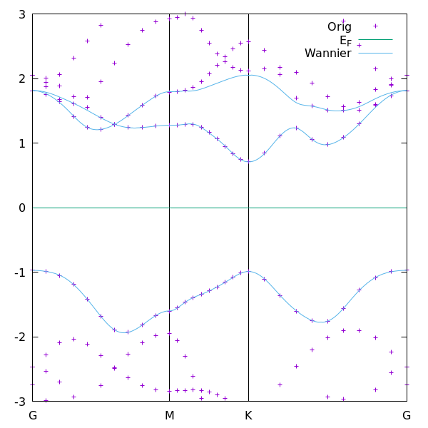
The resulting figure compares the original QE band structure with the Wannier-interpolated band structure.
The goal is to check whether the three-band Wannier model reproduces the DFT bands in the energy region of interest.
If the agreement is good, it means that we have successfully constructed a compact tight-binding model for monolayer MoS2.
As shown in the figure, the Wannier-interpolated bands reproduce the target DFT bands reasonably well, although one band shows a small deviation due to band entanglement. A detailed discussion of this deviation is provided on the next page.
What should we learn from this example?
This example shows the basic logic of building a Wannier tight-binding model:
- calculate the DFT electronic structure;
- choose physically meaningful orbital projections;
- define frozen and outer energy windows;
- construct Wannier functions;
- compare Wannier-interpolated bands with DFT bands.
The most important lesson is that Wannier90 is not just a band-fitting tool. It creates a physically interpretable real-space Hamiltonian. Once we have this Hamiltonian, we can use it for many further calculations: band interpolation, Berry curvature, optical properties, excitons, topological analysis, transport calculations, and more.
In this MoS2 example, the final model is especially elegant: three important bands are described by three localized Mo-centered d-like Wannier functions. This gives us a simple but powerful tight-binding representation of the low-energy electronic structure of monolayer MoS2.