Monolayer MoS2 example: 11-orbital Wannier model
- 1. Generate the k-mesh
- 2. Run the self-consistent QE calculation
- 3. Calculate the QE band structure
- 4. Re-run the SCF calculation before Wannier90
- 5. Prepare the Wannier90 input file
- 6. Choose the orbital projections
- 7. Why does the 11-orbital model work better?
- 8. Define the frozen energy window
- 9. Run Wannier90 preprocessing
- 10. Run pw2wannier90.x
- 11. Run Wannier90
- 12. Check the Wannier90 output
- 13. Wannier centers and spreads
- 14. Visualizing the Wannier functions
- 15. The real-space Hamiltonian: d_hr.dat
- 16. Plot the band structure
- 17. What should we learn from this example?
In the previous example, we built a minimal three-band Wannier model for monolayer MoS2 using only three Mo d-orbitals:
$$d_{z^2}, \quad d_{xy}, \quad d_{x^2-y^2}$$
That model is very useful pedagogically because it is compact and physically transparent. However, it also has a limitation: the selected three bands are partially entangled with nearby DFT bands. As a result, one of the Wannier-interpolated bands may slightly deviate from the target DFT band.
In this example, we build a larger and more robust Wannier model. Instead of using only three Mo d-orbitals, we include:
$$5 \text{ Mo } d\text{-orbitals}$$
and
$$3 \text{ S } p\text{-orbitals for each sulfur atom}$$
Since monolayer MoS2 has one Mo atom and two S atoms in the unit cell, the total number of Wannier functions is
$$5 + 3 + 3 = 11$$
Therefore, this example constructs an 11-orbital tight-binding model for monolayer MoS2.
The important advantage of this model is that these 11 bands form a more complete and better separated group of bands. Because the target band manifold is less entangled with the surrounding bands, Wannier90 can construct a much more accurate interpolation.
You can download the required input files for this example here.
1. Generate the k-mesh
As in the previous example, we first generate a uniform k-mesh using the kmesh.pl utility from the Wannier90/utility/ folder:
kmesh.pl 15 15 1
This creates a $15 \times 15 \times 1$ k-point mesh. Since monolayer MoS2 is a two-dimensional system, only one k-point is used in the out-of-plane direction.
The generated k-points should be inserted into the QE input file:
scf.in
It is important that exactly the same k-mesh is used later in the Wannier90 input file.
2. Run the self-consistent QE calculation
Run the self-consistent DFT calculation:
pw.x < scf.in > scf.out
This step calculates the ground-state charge density. The resulting charge density will be used for the following band-structure and Wannier90 calculations.
3. Calculate the QE band structure
Next, calculate the band structure with Quantum ESPRESSO:
pw.x < bands.in > bands.out bands.x < bandsx.in > bandsx.out
In bands.in, we use the automatic generation of the high-symmetry k-path
$$
\Gamma \rightarrow M \rightarrow K \rightarrow \Gamma.
$$
The corresponding block is:
K_POINTS crystal_b
4
gG   10
M    10
K    10
gG   1
Here, 4 is the total number of high-symmetry points. The number after each point tells QE how many intermediate points should be generated between this point and the next high-symmetry point.
This QE band structure will be used as the reference for checking the Wannier interpolation.
4. Re-run the SCF calculation before Wannier90
Before running Wannier90, we need to run the QE SCF calculation again:
pw.x < scf.in > scf.out
This is done because the QE band-structure calculation may modify or overwrite files required by pw2wannier90.x.
To speed up this calculation, we can restart from the previously calculated charge density by adding:
&electrons
    startingpot = 'file
 /
This tells QE to read the existing potential from file instead of starting completely from scratch.
5. Prepare the Wannier90 input file
The main Wannier90 input file is:
d.win
As before, the same k-mesh generated by kmesh.pl and used in scf.in must also be inserted into d.win.
We also need to provide the same high-symmetry path for plotting the Wannier-interpolated bands. It is best to take the actual k-point coordinates from the QE output and insert them into d.win:
begin kpoint_path
G 0.0       0.0      0.0
M 0.5       0.0      0.0
M 0.5       0.0      0.0
K 0.666667 -0.333333 0.0
K 0.666667 -0.333333 0.0
G 0.0       0.0      0.0
end kpoint_path
This ensures that the QE bands and the Wannier-interpolated bands are plotted along the same path in reciprocal space.
6. Choose the orbital projections
In this example, we use all five Mo (d)-orbitals and all three (p)-orbitals on each S atom:
begin projections
Mo:d
S:p
end projections
This gives
$$ 5 \text{ Mo } d\text{-orbitals} + 3 \text{ S } p\text{-orbitals} + 3 \text{ S } p\text{-orbitals} = 11 \text{ Wannier functions}$$
This basis is much larger than the three-orbital model, but it is also more complete. It describes not only the Mo-dominated states near the band gap, but also the sulfur p-states that participate in bonding and hybridization.
This is why the 11-orbital model usually gives a much better band interpolation over a wider energy range.
7. Why does the 11-orbital model work better?
The most important difference between this example and the previous three-band example is the structure of the target band manifold.
In the three-band model, the target bands are close to other DFT bands. They are partially entangled, so Wannier90 has to choose a smooth three-dimensional subspace from a complicated group of bands. This can lead to small deviations or band-switching behavior.
In the present 11-orbital model, the situation is much better. The selected 11 bands form a larger and more naturally separated group. Since this group is better isolated from the surrounding bands, Wannier90 does not have to solve such a difficult disentanglement problem.
This is an important practical lesson:
$$\text{A minimal model is simpler,}$$
but
$$\text{a larger model can be more stable and accurate.}$$
The 11-orbital model is less minimal, but it is much more robust. It gives Wannier90 enough orbital degrees of freedom to describe the relevant electronic states without forcing the program to artificially compress the physics into too small a basis.
8. Define the frozen energy window
For this model, the frozen window is chosen to contain all 11 target bands:
dis_froz_min  = -7.8
dis_froz_max  =  4.0
The frozen window tells Wannier90 that all bands inside this energy range must be reproduced.
Because we now use 11 Wannier functions, the frozen window can contain 11 bands at each k-point. This is one of the reasons why the 11-orbital model is easier to construct than the three-orbital model. We are no longer trying to force a complicated band manifold into only three Wannier functions.
In practice, the frozen window should be chosen so that it includes the target 11-band group but does not unnecessarily include additional bands outside this group.
9. Run Wannier90 preprocessing
Run Wannier90 in preprocessing mode:
wannier90.x -pp d
This command reads the input file:
d.win
and generates the auxiliary files required by the QE–Wannier90 interface.
10. Run pw2wannier90.x
Now run:
pw2wannier90.x -in pw2wan.in
This program reads the QE data and computes the matrices needed by Wannier90, including the overlap and projection matrices.
In simple words, this step transfers the DFT wave-function information from Quantum ESPRESSO to Wannier90.
11. Run Wannier90
Now run the main Wannier90 calculation:
wannier90.x d
This command again uses the same input file:
d.win
Wannier90 constructs the optimized Wannier functions, calculates the tight-binding Hamiltonian, and produces the Wannier-interpolated band structure.
The main output file is:
d.wout
This file contains detailed information about the disentanglement and localization procedures.
12. Check the Wannier90 output
After the calculation, open:
d.wout
This file contains the most important information about the result, including:
- convergence of the spread
- final Wannier centers
- individual Wannier spreads
- total spread
- information about disentanglement
A good calculation should show stable final spreads and physically meaningful Wannier centers.
13. Wannier centers and spreads
In d.wout, Wannier90 prints the final centers and spreads of the Wannier functions. For this example, the output may look like:
                                    x          y          z
WF centre and spread    1  ( -0.000110, -0.005026,  3.020251 )     1.54172012
WF centre and spread    2  (  0.000153,  0.045406,  3.020251 )     1.83557467
WF centre and spread    3  ( -0.000329, -0.045535,  3.020251 )     1.83352507
WF centre and spread    4  (  0.000516,  0.119880,  3.020251 )     1.69736081
WF centre and spread    5  ( -0.000848, -0.113467,  3.020251 )     1.70068481
WF centre and spread    6  (  1.591188,  0.911559,  1.353363 )     1.73996114
WF centre and spread    7  (  1.591423,  0.905479,  1.500671 )     1.67444195
WF centre and spread    8  (  1.591345,  0.934700,  1.500455 )     1.67520821
WF centre and spread    9  (  1.591193,  0.911562,  4.687140 )     1.73996212
WF centre and spread   10  (  1.591417,  0.905479,  4.539830 )     1.67444574
WF centre and spread   11  (  1.591345,  0.934696,  4.540046 )     1.67521074
The first five Wannier functions have centers close to the Mo atom. These functions correspond to the five Mo d-like orbitals.
The next three Wannier functions are centered close to one sulfur atom and correspond to sulfur p-like orbitals.
The last three Wannier functions are centered close to the other sulfur atom and also correspond to sulfur p-like orbitals.
Thus, the centers confirm the physical interpretation of the model:
$$
\text{WFs 1–5} \rightarrow \text{Mo } d\text{-like orbitals},
$$
$$
\text{WFs 6–8} \rightarrow \text{lower S } p\text{-like orbitals},
$$
$$
\text{WFs 9–11} \rightarrow \text{upper S } p\text{-like orbitals}.
$$
This is a very important check. The Wannier functions are not just numerical fitting functions. Their centers and shapes should correspond to the orbitals that we used as projections.
14. Visualizing the Wannier functions
Wannier90 can write files for visualizing the Wannier functions. In this example, the files are:
d_00001.xsf
d_00002.xsf
...
d_00011.xsf
These files can be opened in visualization programs such as VESTA or XCrySDen.
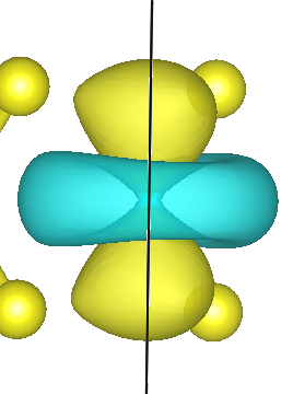
The first Wannier function is $d_{z^2}$-like and is centered on the Mo atom
The second Wannier function shows stronger hybridization between Mo d- and S p-character
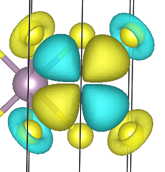
This is physically reasonable. In a real crystal, Wannier functions are not always pure atomic orbitals. They often contain hybridization tails on neighboring atoms. This is especially true in covalent or partially covalent materials such as MoS2.
Therefore, a Wannier function can be “Mo-centered” while still having visible weight on the surrounding sulfur atoms.
15. The real-space Hamiltonian: d_hr.dat
One of the most important output files produced by Wannier90 is:
d_hr.dat
This file contains the matrix elements of the tight-binding Hamiltonian in the Wannier basis:
$$H_{mn}(\mathbf{R}_C)$$
Here, m and n are Wannier function indices, and $\mathbf{R}_C$ is a lattice vector connecting unit cells.
This file is extremely important because it is the actual tight-binding model generated by Wannier90. It can be used later for band interpolation, model Hamiltonian calculations, Berry curvature, transport, optical properties, excitons, and many other applications.
The beginning of d_hr.dat contains general information. Line 2 gives the number of Wannier functions:
11
Line 3 gives the number of lattice vectors $\mathbf{R}_C$. In this example, for a $15 \times 15 \times 1$ k-mesh, this number is:
225
Then follow the degeneracy numbers. After that, the Hamiltonian matrix elements are printed in the form:
    i    j    k    m    n     Re Hmn      Im Hmn
   -9   -5    0    1    1    0.000207   -0.000000
   -9   -5    0    2    1   -0.000136   -0.000000
   -9   -5    0    3    1    0.000033   -0.000000
The first three integers,
i j k
define the lattice cell vector:
$$\mathbf{R}_C = i\mathbf{a}_1 + j\mathbf{a}_2 + k\mathbf{a}_3$$
The next two integers,
m n
are the Wannier function indices.
The final two numbers are the real and imaginary parts of the Hamiltonian matrix element:
$$
\mathrm{Re}(H_{mn}(\mathbf{R}_C))
\quad
\mathrm{Im}(H_{mn}(\mathbf{R}_C)).
$$
Thus, each line gives one hopping or onsite matrix element between Wannier functions.
For example, if
$$
\mathbf{R}_C = 0
$$
and
$$
m = n,
$$
then the matrix element corresponds to an onsite energy of the m-th Wannier orbital.
If
$$
\mathbf{R}_C \neq 0
$$
or
$$
m \neq n,
$$
then the matrix element describes hopping or hybridization between different orbitals or different unit cells.
This is the central output of Wannier90: it converts the DFT electronic structure into a compact real-space Hamiltonian.
16. Plot the band structure
Finally, plot the band structure using:
gnuplot plot.gnu
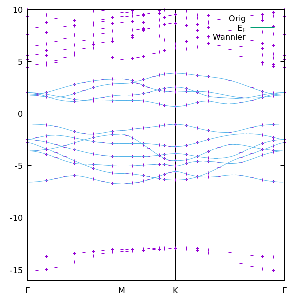
The figure compares the QE band structure with the Wannier-interpolated band structure obtained from the 11-orbital model.
In contrast to the minimal three-band model, the 11-orbital model usually reproduces the DFT bands very well over a much wider energy range. This happens because the selected 11 bands form a better separated band manifold and because the Wannier basis contains the main Mo d- and S p-orbital characters.
17. What should we learn from this example?
This example demonstrates an important principle of Wannier modeling.
The minimal three-orbital model is useful because it gives a simple and intuitive picture of the low-energy Mo d-states near the band gap. However, because it uses only three orbitals, it may have difficulty when the target bands are entangled with nearby bands.
The 11-orbital model is larger, but it is more complete. It includes all Mo d-orbitals and all S p-orbitals in the unit cell. As a result, the selected band manifold is better represented, and the Wannier interpolation becomes much more accurate.
The comparison between the two examples teaches an important practical lesson:
A smaller Wannier model is simpler and easier to interpret, but a larger Wannier model is often more accurate and more robust.
For real research calculations, one should always choose the Wannier basis according to the goal of the calculation.
If the goal is a simple low-energy model, a small number of Wannier functions may be sufficient.
If the goal is accurate band interpolation over a wider energy range, or if the bands are strongly entangled, a larger Wannier basis is usually the better choice.
In this MoS2 example, the 11-orbital model provides an excellent and physically meaningful tight-binding representation of the DFT band structure.