- Green’s Function Notation
- Convention Used in This Tutorial
- Propagators: Green Functions in Diagrammatic Methods
- Time Flow and Fermion Flow
- Why Arrow Conventions Matter
- Interactions: Bare and Screened Coulomb Potentials
- Elementary Building Units: Bare Propagator $G_0$ and Bare Interaction $v$
- Self-Energy Insertions and Polarization Bubbles
- Two Basic Composite Structures: Polarization and Exchange
Feynman diagrams provide a graphical language for representing propagation and interaction processes in quantum systems. They are widely used in quantum field theory, condensed matter physics, nuclear physics, and quantum chemistry.
In this tutorial, we focus on their application to electronic many-body theory. In this context, Feynman diagrams provide a natural way to represent Green’s functions, self-energies, polarization functions, and screened interactions. While this tutorial focuses on electronic many-body theory, Feynman diagrams are used much more broadly; see Examples of Feynman Diagram Applications Across Disciplines for an overview.
Condensed matter systems are especially rich examples because electrons do not propagate in isolation. Their motion is modified by interactions with other electrons, screening by the surrounding medium, quasiparticle formation, and collective excitations. Diagrammatic methods allow these effects to be represented visually and translated into mathematical expressions.
Feynman diagrams are therefore not just pictures. They are compact graphical representations of mathematical objects in many-body theory. To read them correctly, we first introduce the most important object in this graphical language: the Green’s function, or propagator.
Green’s Function Notation
The field operator
$$\widehat{\psi}^{\dagger}(1)$$
creates an electron at point 1, while
$$\widehat{\psi}(2)$$
annihilates an electron at point 2.
For the diagrams considered below, time flows from left to right, and we choose
$$t_2>t_1.$$
Thus, point 1 is the initial point and point 2 is the final point. The particle is created at point 1, propagates through the system, and is annihilated at point 2.
The corresponding time-ordered Green’s function is
$$G(1,2) = -i \left\langle T \left[ \widehat{\psi}(2) \widehat{\psi}^{\dagger}(1) \right] \right\rangle.$$
The time-ordering operator $T$ arranges field operators according to their time arguments, placing the operator with the later time to the left. Because electrons are fermions, exchanging two field operators introduces an additional minus sign.
For $t_2>t_1$, the operators are already in time-ordered form, so this becomes
$$G(1,2) = -i \left\langle \widehat{\psi}(2) \widehat{\psi}^{\dagger}(1) \right\rangle.$$
Convention Used in This Tutorial
Throughout this tutorial, the arguments of a Green’s function follow the direction of propagation:
$$G(1,2) \equiv \text{propagation from point }1\text{ to point }2.$$
Thus, the first argument labels the initial point, where the particle is created, and the second argument labels the final point, where it is annihilated:
$$1\longrightarrow 2.$$
More generally,
$$G(a,b) = -i \left\langle T \left[ \widehat{\psi}(b) \widehat{\psi}^{\dagger}(a) \right] \right\rangle $$
describes propagation from a to b.
Many textbooks use the alternative notation
$$G(b,a) = -i \left\langle T \left[ \widehat{\psi}(b) \widehat{\psi}^{\dagger}(a) \right] \right\rangle,$$
where the arguments follow the order of the field operators rather than the direction shown in the diagram. The two conventions describe the same physical process. In this tutorial, we use the propagation-order convention consistently so that the notation follows the diagrams directly.
Propagators: Green Functions in Diagrammatic Methods
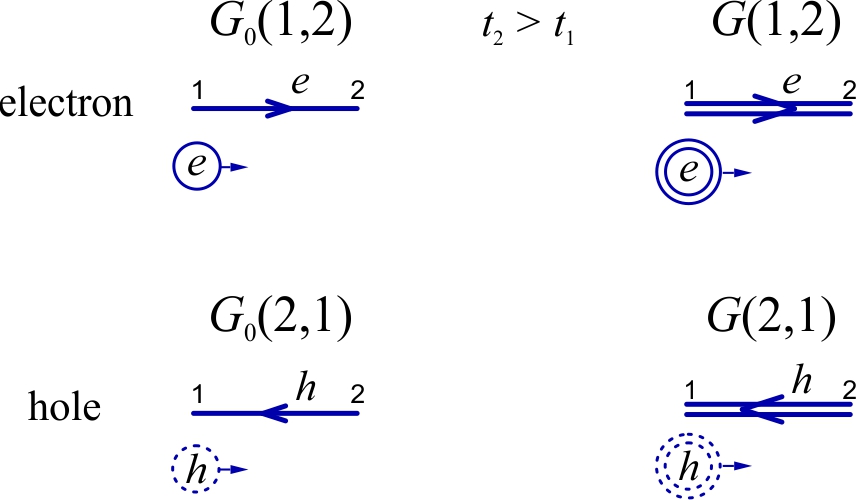
The Green’s function, or propagator, describes how a single-particle excitation propagates from one point to another. In diagrammatic many-body theory, Green’s functions are represented by lines connecting spacetime points.
For a non-interacting system, the propagation is described by the bare Green’s function $G_0$. The corresponding Feynman diagram is a single line connecting two points.
The external points represent spacetime coordinates. The line connecting these points represents single-particle propagation between them.
The interacting, or dressed, Green’s function $G$ describes propagation in the presence of interactions. In this case, the particle or hole does not propagate freely. Its motion is modified by interactions with the surrounding many-body environment. These interaction effects are encoded through the self-energy $\Sigma$, which collects the corrections due to interaction processes.
Diagrammatically, the dressed Green’s function is often represented by a double line. This double line denotes a dressed single-particle propagator, not two particles.
Thus, $G_0$ represents bare propagation, while $G$ represents dressed propagation.
Physically, replacing $G_0$ by $G$ means that the propagating excitation is no longer isolated. It is dressed by interactions with other electrons, collective excitations, screening effects, and the surrounding many-body medium.
Time Flow and Fermion Flow
The arrows on fermionic propagator lines indicate the direction of fermion flow, which does not always coincide with the direction of time.
Throughout this tutorial, we assume $t_2>t_1,$ so that time flows from point 1 to point 2.
Electron propagation
Using the propagation-order convention introduced above,
$$G_0(1,2) = -i \left\langle T \left[ \widehat{\psi}(2) \widehat{\psi}^{\dagger}(1) \right] \right\rangle.$$
Since $t_2>t_1$, the operators are already time ordered:
$$G_0(1,2) = -i \left\langle \widehat{\psi}(2) \widehat{\psi}^{\dagger}(1) \right\rangle. $$
An electron is created at point 1 and annihilated at point 2. Thus, both the electron and the fermion-flow arrow move from 1 to 2:
$$1\xrightarrow{\ e\ }2.$$
Hole propagation
For the reversed fermion flow,
$$G_0(2,1) = -i \left\langle T \left[ \widehat{\psi}(1) \widehat{\psi}^{\dagger}(2) \right]\right\rangle. $$
Because the operator at the later time must be moved to the left, time ordering introduces a fermionic minus sign. Therefore,
$$G_0(2,1) = +i \left\langle \widehat{\psi}^{\dagger}(2) \widehat{\psi}(1) \right\rangle.$$
At point 1, an electron is removed from an occupied state, creating a hole. At point 2, the electron is restored and the hole disappears. The hole therefore propagates forward in time from 1 to 2, while the fermion-flow arrow points in the opposite direction:
$$1\xleftarrow{\ \text{fermion flow}\ }2.$$
Thus, for $t_2>t_1$,
$$G_0(1,2) \quad\longleftrightarrow\quad \text{electron propagation from }1\text{ to }2, $$
whereas
$$G_0(2,1)\quad\longleftrightarrow\quad \text{hole propagation from }1\text{ to }2.$$
The key point is that time always flows from 1 to 2, while the arrow on the fermionic line follows fermion flow: it points forward for an electron and backward for a hole.
Why Arrow Conventions Matter
The arrows on fermionic propagator lines are part of the mathematical structure of a Feynman diagram. They indicate fermion flow and help determine how Green’s-function arguments are connected through the diagram.
The direction of a fermionic arrow should not be confused with the distinction between different types of Green’s functions. Here we use the time-ordered Green’s function. Retarded, advanced, lesser, and greater Green’s functions are defined by different time-ordering rules and boundary conditions, not by reversing the arrow on a line. These other Green’s functions become important in more advanced applications, but they are not needed for the diagrammatic convention introduced here.
In this tutorial, we use the convention
$$t_2>t_1,$$
so time increases from point 1 to point 2. The arrows on fermionic lines indicate fermion flow. With this convention,
$$G_0(1,2)$$
describes electron propagation from 1 to 2, while
$$G_0(2,1)$$
describes hole propagation from 1 to 2. In the hole case, the physical hole moves forward in time, but the fermion-flow arrow points in the opposite direction.
Different authors may use different arrow conventions. In some diagrams, arrows indicate fermion-number flow; in others, they may indicate charge flow, quasiparticle propagation, or simply the orientation in which the propagator is read. Also, many Feynman diagrams are drawn as topological graphs rather than spacetime pictures, so left-to-right placement does not always mean increasing time.
For this reason, before reading diagrams from another source, one should identify the author’s convention for the direction of time, the meaning of arrows, and the ordering of Green’s-function arguments. Once these conventions are fixed, the diagram can be translated into a mathematical expression unambiguously.
Interactions: Bare and Screened Coulomb Potentials
1. Coulomb Interaction in Many-Body Theory
In atomic units, and omitting material-dependent background dielectric factors, the bare Coulomb interaction can be written as:
- $$v(\mathbf{r}-\mathbf{r}') = \frac{1}{|\mathbf{r}-\mathbf{r}'|}$$
In momentum space, for a three-dimensional homogeneous system:
- $$v(\mathbf{q}) = \frac{4\pi}{q^2}$$
This is the bare Coulomb interaction — no screening, just the fundamental electrostatic interaction.
2. Bare Coulomb Interaction (Single Wiggly Line)
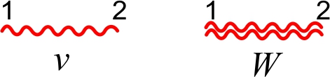
In Feynman diagrams, the bare Coulomb interaction is represented by a single wiggly line connecting two electron lines. Why wiggly? It distinguishes it from straight fermion lines and indicates a bosonic mediator (photon in quantum electro-dynamics (QED) or Coulomb field in condensed matter). In the non-relativistic condensed-matter approximation, the bare Coulomb interaction is usually treated as instantaneous, so $v(\mathbf q)$ has no explicit frequency dependence.
3. Screened Coulomb Interaction (Double Wiggly Line)
In a medium, electrons polarize the environment, reducing the effective interaction. This gives the screened Coulomb interaction:
- $$W(\mathbf{q},\omega) = \varepsilon^{-1}(\mathbf{q},\omega) v(\mathbf{q}) $$
where $\varepsilon(\mathbf{q},\omega)$ is the dielectric function. This is dynamic (depends on frequency) because screening responds over time.
In diagrams, we use a double wiggly line for $W$ to indicate that the interaction has been screened by the response of the medium. In the random-phase approximation, this screening can be represented as a series of polarization-bubble insertions.
4. Physical Interpretation
Single wiggly line: Instantaneous, unscreened Coulomb force.
Double wiggly line: Effective interaction after accounting for medium response (screening).
Why no direction in Coulomb potential?
1. Coulomb Interaction Represents an Interaction, Not Particle Flow
The wiggly line (single or double) corresponds to the exchange of an interaction, not the propagation of a particle with conserved charge.
Unlike electron Green functions, which describe the motion of a fermion from one point to another (requiring arrows to track particle number and time ordering), the Coulomb line represents a potential field connecting two points.
2. No Charge Flow → No Arrow
For fermionic lines, arrows are essential because:
- they track fermion flow through vertices;
- they distinguish opposite orientations of electron-like and hole-like propagation;
- they help determine the ordering of Green’s-function arguments once the diagrammatic convention is fixed.
For Coulomb interaction:
- It’s an instantaneous (or dynamically screened) potential.
- There is no conserved quantity flowing along the wiggly line.
- The interaction is symmetric: exchanging the two ends does not change the physics.
3. Mathematical Reason
The Coulomb propagator is a scalar function, see Eqs. (2) and (3). There’s no operator that distinguishes “incoming” vs “outgoing” along this line. It’s just a factor in the interaction term.
Distinction between Coulomb interaction in condensed matter diagrams and full electromagnetic propagation in QED
1. Why No Direction for Coulomb Lines in Many-Body Diagrams?
In condensed matter physics, the Coulomb interaction is usually treated in the instantaneous approximation (non-relativistic limit). This means we assume the interaction acts immediately between two electrons, ignoring the finite speed of light. The wiggly line represents the potential, not a real photon traveling through space-time. Therefore, there’s no need to indicate direction — the interaction is symmetric.
2. Where Is Speed of Light Considered?
In full quantum electrodynamics (QED), the mediator of the interaction is the photon, which propagates at the speed of light. In that case, the wiggly line is actually a photon propagator, which includes time dependence and respects causality, just like electron propagators. If you were doing QED diagrams, the wiggly line does represent real propagation at finite speed.
3. Why Condensed Matter Ignores This?
Electron velocities in solids are much smaller than $c$. Retardation effects (finite speed of light) are negligible compared to electronic timescales. So we replace the photon propagator with an instantaneous Coulomb potential Eq. (2). Screening can introduce frequency dependence through the dielectric function $\varepsilon(\mathbf q,\omega)$. This frequency dependence describes the dynamical response of the electronic medium, not necessarily the finite-speed propagation of real photons.
4. If We Include Retardation
In advanced many-body theory, the screened interaction $W(\mathbf{q},\omega)$ may depend on frequency. The frequency dependence of $W$ describes the delayed dynamical response of the electronic medium. It should not generally be identified with electromagnetic retardation associated with the finite speed of light.
5. When Photons Are Explicitly Included
In optics, nonlinear optics, and light–matter interaction studies, photons are treated explicitly. Feynman diagrams then include wiggly lines for photons (similar to QED). These diagrams describe processes like absorption, emission, and scattering. In strong coupling regimes (e.g., polaritons, exciton–photon coupling), photons are part of the Hamiltonian and treated on equal footing with electrons.
Elementary Building Units: Bare Propagator $G_0$ and Bare Interaction $v$
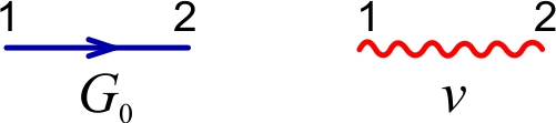
For the electronic many-body problem considered in this tutorial, the perturbative expansion is built from two elementary ingredients: the bare electron propagator $G_0$ and the bare Coulomb interaction $v$.
More general field theories may contain additional propagators and vertices, such as phonon, photon, spin, or bosonic collective fields. Here we focus on the standard electron-electron Coulomb problem.
Why only two elementary building blocks?
In diagrammatic many-body theory, the starting point is a perturbative expansion of the interacting system around a reference system of non-interacting particles. This reference system is described by bare electron propagator $G_0$ and bare Coulomb interaction $v$.
Physical meaning
$G_0$ describes free propagation of electrons, while $v$ describes the bare electron-electron interaction. By repeatedly connecting these blocks, we generate higher-order processes such as exchange, polarization, screening, and vertex corrections.
Why is this universal?
This structure is common in electronic many-body theory because the expansion starts from single-particle propagation and a two-body Coulomb interaction. More general theories may require additional fields, propagators, and vertices.
Self-Energy Insertions and Polarization Bubbles
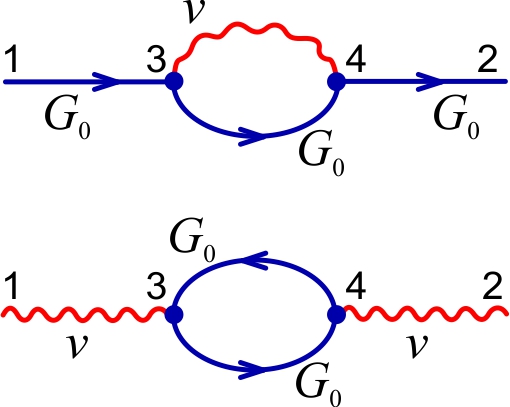
A vertex represents a point in space-time at which propagator and interaction lines are connected according to the interaction term in the Hamiltonian. External points, such as 1 and 2, are fixed by the Green’s function being calculated. Internal vertices, by contrast, describe intermediate interaction events whose positions, times, and other internal variables are not fixed. They must therefore be integrated over.
For example, the internal vertices 3 and 4 shown in the diagrams lead to integrations over $d3 d4$. Two important structures that appear in such expansions are
- $$\int d3 d4 \; G_0(1,3) \; \underbrace{iG_0(3,4)v(4,3)}_{\text{self-energy insertion}} \; G_0(4,2)$$
- $$\int d3 d4 \; v(1,3) \; \underbrace{-iG_0(3,4)G_0(4,3)}_{\text{polarization bubble}} \; v(4,2)$$
Here, numerical prefactors and sign conventions may depend on the precise definition of the Green’s functions and interaction lines, but the diagrammatic structures remain the same.
Although the variables 3 and 4 are integrated over, they still identify the endpoints at which the propagator and interaction lines meet. The interaction line $v(3,4)$ connects two such endpoints. For the bare Coulomb interaction, this line represents a generally nonlocal interaction between the spatial coordinates associated with the two vertices.
The product $G_0(3,4)G_0(4,3)$ forms a closed fermion loop: following the fermionic propagators takes us from 3 to 4 and then back to 3. Together with the factor $-i$, this structure defines the independent-particle polarization,
$$P_0(3,4)=-iG_0(3,4)G_0(4,3).$$
Diagrammatically, it is called a polarization bubble. Physically, it represents a virtual particle-hole fluctuation and generates the screening of the interaction.
By contrast, $iG_0(3,4)v(4,3)$ contains one fermionic propagator and one interaction line. It is therefore not a closed fermion loop. Instead, it defines the first-order exchange, or Fock, self-energy,
$$\Sigma_x(3,4)=iG_0(3,4)v(4,3),$$
which appears as a self-energy insertion in the single-particle propagator. This insertion modifies single-particle propagation through the exchange interaction.
Thus, both expressions contain internal variables arranged in a cyclic pattern, $3\rightarrow4\rightarrow3$, but they represent different diagrammatic objects. The types of lines forming the closed structure determine whether it should be interpreted as a self-energy insertion or as a polarization bubble.
Two Basic Composite Structures: Polarization and Exchange
In the electronic many-body problem, repeated combinations of the bare propagator \(G_0\) and the bare interaction \(v\) generate several important diagrammatic structures.
A polarization bubble contains two fermionic propagators,
$$G_0(3,4)G_0(4,3),$$
forming a closed particle-hole loop. This structure describes density fluctuations of the electronic system and contributes to screening of the bare Coulomb interaction.
An exchange self-energy insertion contains a fermionic propagator connected by the bare interaction,
$$G_0(3,4)v(4,3).$$
This structure modifies single-particle propagation through exchange interaction. It should be distinguished from the polarization bubble: it is not a screening loop, and it is not usually classified as a correlation correction beyond Hartree.
These two structures enter different physical quantities. Polarization bubbles build the screened interaction $W$, while exchange-like self-energy insertions contribute to the self-energy $\Sigma$.