- Physical meaning
- Where does the Dyson equation come from?
- Integral form
- Diagrammatic representation
- Repeated self-energy insertions
- Dressed propagation
- More advanced treatment
Throughout this section, the Hamiltonians, Green’s functions, and self-energy are operators. In full notation, they are written as
$$\widehat{H}_0, \qquad \widehat{G}_0(E), \qquad \widehat{\Sigma}(E), \qquad \widehat{G}(E).$$
Here, $E$ is an energy variable, so expressions such as $E-H_0$ are shorthand for
$$E\widehat{I}-\widehat{H}_0,$$
where $\widehat{I}$ is the identity operator.
To keep the notation simple, operator hats, the explicit energy dependence, and the identity operator will be omitted below.
Suppose that $G_0$ describes propagation in a chosen reference system. This reference may correspond to a noninteracting particle or to a particle moving in an effective mean-field potential.
Interactions change this propagation. Their combined effect is represented by the self-energy
$$\Sigma.$$
The resulting interacting Green’s function is denoted by
$$G.$$
The Dyson equation connects these three quantities.
Physical meaning
The full propagation can be divided into two possibilities.
First, the particle may propagate according to the reference Green’s function $G_0$.
Second, it may propagate according to $G_0$, undergo a self-energy process $\Sigma$, and then continue propagating according to the full Green’s function $G$.
This gives
- $$G = G_0 + G_0\Sigma G$$
The two terms have a simple interpretation:
- $G_0$ describes propagation without a self-energy insertion, while
- $G_0\Sigma G$ describes propagation that includes an interaction process.
Where does the Dyson equation come from?
Let the reference Hamiltonian be $H_0$.
Its Green’s function is
$$G_0 = \left( E-H_0 \right)^{-1}.$$
Interactions modify the propagation of the particle. Their effect is represented by the self-energy $\Sigma$.
The full Green’s function is therefore
$$G = \left( E-H_0-\Sigma \right)^{-1}.$$
From the definition of $G_0$,
$$G_0^{-1} = E-H_0.$$
Therefore, the full Green’s function can be written as
$$G = \left( G_0^{-1}-\Sigma \right)^{-1}.$$
Equivalently,
$$G^{-1} = G_0^{-1}-\Sigma.$$
Now add $\Sigma$ to both sides:
$$G_0^{-1} = G^{-1}+\Sigma.$$
Multiplying from the left by $G_0$ and from the right by $G$, we obtain
$$G_0G_0^{-1}G = G_0G^{-1}G + G_0\Sigma G.$$
Since
$$G_0G_0^{-1}=1$$
and
$$G^{-1}G=1,$$
this becomes
$$G = G_0 + G_0\Sigma G$$
This is the Dyson equation.
Integral form
In real space and time, the Dyson equation becomes an integral equation.
A composite label such as 1 collects the variables used in the chosen representation. For example,
$$ 1\equiv (\mathbf r_1,t_1,\sigma_1),$$
where $\mathbf r_1$ is position, $t_1$ is time, and $\sigma_1$ is a spin index.
The Dyson equation is then
- $$G(1,2) = G_0(1,2) + \int d3 d4 G_0(1,3) \Sigma(3,4) G(4,2) $$
The labels 3 and 4 represent intermediate variables over which the equation is integrated.
The second term describes the following sequence:
$$1 \xrightarrow{G_0} 3 \xrightarrow{\Sigma} 4 \xrightarrow{G} 2.$$
The particle propagates from point 1 to point 3 according to the reference propagator $G_0$. It then undergoes an interaction process represented by the self-energy $\Sigma(3,4)$, after which it propagates from point 4 to point 2 according to the full propagator $G$.
Products such as
$$G_0\Sigma G $$
therefore represent convolutions over intermediate spatial, temporal, spin, orbital, or other internal variables.
After Fourier transformation, the same equation may be expressed in momentum and frequency space.
Diagrammatic representation
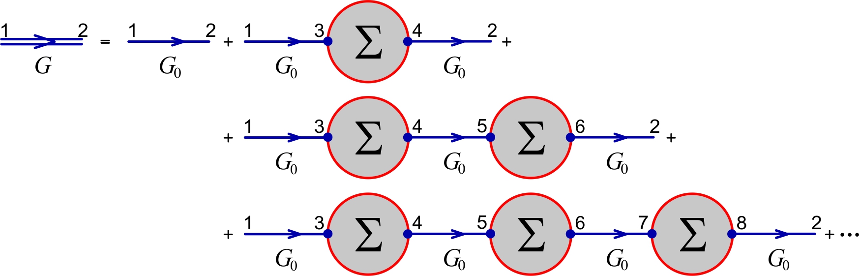
The Dyson equation (1) has a simple graphical interpretation.

In the convention used in this tutorial:
- a single solid line with an arrow represents the reference propagator $G_0$;
- a double or dressed line with an arrow represents the full propagator $G$;
- a self-energy insertion represents $\Sigma$.
The Dyson equation (1) states that the dressed propagator $G$ is equal to the reference propagator $G_0$ plus a propagation process $G_0\Sigma G$ containing a self-energy insertion $\Sigma$, followed by further dressed propagation $G$.
The arrow indicates the direction associated with particle propagation in the chosen diagrammatic convention.
The self-energy insertion $\Sigma$ represents an individual interaction contribution. Repeated self-energy insertions are generated automatically by the Dyson equation, as shown below.
In the diagrams shown here, time flows from left to right, and the arrows illustrate electron propagation. Reversing the arrows gives the corresponding hole-propagation diagram. More generally, the full time-ordered Green’s function contains both electron and hole contributions.
Repeated self-energy insertions
The full Green’s function appears on both sides of the Dyson equation:
$$G = G_0 + G_0\Sigma G.$$
We can substitute the same expression for $G$ on the right-hand side:
$$G = G_0 + G_0\Sigma \left( G_0+G_0\Sigma G \right).$$
Expanding the expression gives
$$G = G_0 + G_0\Sigma G_0 + G_0\Sigma G_0\Sigma G.$$
Repeating the substitution again produces
$$ G = G_0 + G_0\Sigma G_0 + G_0\Sigma G_0\Sigma G_0 + G_0\Sigma G_0\Sigma G_0\Sigma G.$$
Continuing indefinitely, we obtain
$$G = G_0 + G_0\Sigma G_0 + G_0\Sigma G_0\Sigma G_0 + G_0\Sigma G_0\Sigma G_0\Sigma G_0 +\cdots$$
This is the iterative expansion of the Dyson equation.
Diagrammatically, it represents:
- propagation without a self-energy insertion $G_0$;
- propagation with one self-energy insertion $G_0\Sigma G_0$;
- propagation with two self-energy insertions $G_0\Sigma G_0\Sigma G_0$;
- propagation with three self-energy insertions $G_0\Sigma G_0\Sigma G_0\Sigma G_0$;
- and so on.
The Dyson equation therefore resums an infinite sequence of repeated insertions of the chosen self-energy.
It is important to distinguish this iterative expansion from an ordinary perturbation expansion in a small interaction parameter.
This series is organized by the number of self-energy insertions. It is not necessarily an expansion in a small interaction strength, because the self-energy $\Sigma$ may already contain several interaction processes.
The series is not usually truncated term by term. Instead, the Dyson equation sums all repeated insertions into the compact expression
$$G = \left( G_0^{-1}-\Sigma \right)^{-1}.$$
In practical calculations, one approximates the self-energy $\Sigma$ and then solves the Dyson equation to obtain $G$.
Dressed propagation
The reference propagator $G_0$ describes how a particle propagates in the chosen reference system.
The full propagator $G$ describes how this propagation is modified by interactions.
Such an interacting excitation is called a dressed particle. The word “dressed” means that the particle is accompanied by the response of its environment.
For example, an electron moving through a material can:
- polarize the surrounding electrons;
- interact with collective charge excitations;
- emit or absorb phonons;
- scatter from other particles;
- interact with defects or impurities.
These processes modify the electron’s propagation and are collected into the self-energy $\Sigma$.
If the dressed excitation remains sufficiently long-lived and produces a well-defined spectral peak, it can be described as a quasiparticle.
The Dyson equation does not determine the self-energy itself. It only shows how a chosen self-energy modifies the Green’s function. The physical meaning and construction of $\Sigma$ will be discussed in the next section.
More advanced treatment
For a more detailed discussion of the operator derivation, different representations, retarded Green’s functions, proper self-energy, and Dyson resummation, see: More advanced aspects of the Dyson equation
Next: Part III — Self-Energy