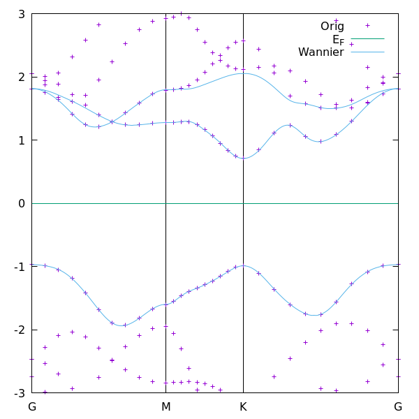
The comparison between the original QE bands and the Wannier-interpolated bands is one of the most important checks in any Wannier90 calculation. In this example, the agreement is generally good: the three Wannier bands reproduce the main low-energy structure of monolayer MoS2 near the band gap. However, one can notice that one of the Wannier bands does not perfectly follow the desired DFT band along the whole high-symmetry path. In some region, it slightly moves toward a neighboring band.
This is not an unusual problem. In fact, it is one of the most common situations that students encounter when they start working with Wannier90.
The reason is that, in this example, we are trying to build a very compact model with only three Wannier functions. These three Wannier functions are chosen to represent the three most important bands near the gap:
$$\text{VBM}, \quad \text{CBM}, \quad \text{CBM+1}$$
Physically, this is a very attractive model because these bands are mainly formed by three Mo d-orbitals:
$$d_{z^2}, \quad d_{xy}, \quad d_{x^2-y^2}$$
Therefore, the model is simple, minimal, and easy to interpret. However, this simplicity has a price. The three target bands are not perfectly isolated from all other DFT bands throughout the whole Brillouin zone. In some regions of k-space, especially away from the immediate band edge, nearby bands may come close in energy or have similar orbital character. When this happens, Wannier90 has to decide which three-dimensional subspace should be selected from a larger group of entangled DFT bands.
This is the essence of the disentanglement problem.
In an ideal situation, the three target bands would be separated from all other bands by clear energy gaps at every k-point. Then Wannier90 would have a simple task: it would just follow this isolated group of three bands. But in the present three-band MoS₂ model, the target bands are partially entangled with other bands. As a result, Wannier90 does not simply “copy” three visually selected DFT bands. Instead, it constructs the smoothest three-dimensional subspace that is compatible with the chosen projections and energy windows.
This distinction is very important.
The Wannier-interpolated bands are not obtained by manually tracing DFT bands one by one. They are obtained from a smooth real-space Hamiltonian built from localized Wannier functions. Therefore, if a neighboring DFT band has similar orbital character, or if the desired band is not protected by the frozen window, the Wannier band may partially follow the neighboring state. The resulting band may still be smooth and physically meaningful, but it may not coincide exactly with the DFT band that we wanted to reproduce.
This is why one of the Wannier bands in the figure can appear to “switch” or drift toward another DFT band.
The role of the frozen window
The first parameter to check is the frozen energy window:
dis_froz_min  = -1.90
dis_froz_max  =  1.53
The frozen window tells Wannier90 which states must be reproduced exactly. In simple words, it says:
The bands inside this energy interval are mandatory.
For a model with
num_wann = 3
the frozen window must contain no more than three bands at any k-point. If it contains four or more bands at some k-point, Wannier90 cannot force all of them into a three-dimensional Wannier subspace and will stop with an error.
If the problematic band moves outside the frozen window in some region of the Brillouin zone, then Wannier90 is no longer forced to reproduce it exactly. In that case, the program may choose a nearby band or a mixture of nearby bands that gives a smoother and more localized Wannier representation.
Therefore, if one Wannier band does not follow the desired DFT band, the first practical step is to check whether this desired band is fully included in the frozen window.
One can try to slightly increase the upper boundary:
dis_froz_max = 1.70
or
dis_froz_max = 1.80
and repeat the calculation. If the agreement improves, then the problem was likely that the desired band was not sufficiently protected by the frozen window.
However, this procedure has a strict limitation. If increasing dis_froz_max includes more than three DFT bands at some k-point, Wannier90 will stop. This means that a three-band model cannot exactly freeze all the desired states in that energy range. In this case, the problem is not just numerical. It means that the minimal three-band subspace is genuinely entangled with other bands.
The role of the outer window
The second important parameter is the outer disentanglement window:
dis_win_min   = -5.0
dis_win_max   =  4.5
The outer window defines the set of DFT bands from which Wannier90 is allowed to construct the optimal Wannier subspace.
The frozen window says:
These states must be included.
The outer window says:
Search for the best subspace within this larger energy range.
If the outer window is too narrow, the program may not have access to all relevant states needed to construct a smooth Wannier subspace. In that case, expanding the outer window can help. For example, one may try:
dis_win_min = -5.0
dis_win_max = 5.0
or
dis_win_min = -6.0
dis_win_max = 5.0
However, a wider outer window is not always better. If the outer window becomes too large, many irrelevant high-energy or low-energy states enter the disentanglement procedure. This can make the problem more difficult and may even worsen the result.
Therefore, the outer window should be wide enough to include the relevant nearby bands, but not so wide that it introduces many unrelated states.
Why simply increasing the number of iterations may not solve the problem
Another natural idea is to increase the number of disentanglement and localization iterations:
dis_num_iter = 1000
num_iter     = 1000
or even:
dis_num_iter = 2000
num_iter     = 2000
This is a useful test. If the calculation has not converged, increasing the number of iterations may improve the result.
However, if the problem is caused by the physical entanglement of the target bands with other bands, increasing the number of iterations alone will not fully solve it. The calculation may converge perfectly, but it will converge to the best three-dimensional subspace available under the given constraints. If three Wannier functions are not enough to describe the chosen energy range, no number of iterations can completely fix the model.
This is an important lesson: convergence of the Wannier90 algorithm does not automatically mean that the chosen model is physically complete.
Check the orbital character
A very useful diagnostic is to inspect the orbital-projected band structure or the projected density of states. In Quantum ESPRESSO, this can be done using:
projwfc.x
The purpose is to answer the following question:
Does the problematic DFT band have the orbital character included in our Wannier basis?
In this tutorial, our basis contains only:
Mo:dz2
Mo:dxy
Mo:dx2-y2
If the problematic band has strong contribution from other orbitals, for example
Mo:dxz
Mo:dyz
S:px
S:py
S:pz
then the three-orbital model is incomplete. In that case, the deviation of the Wannier band is not surprising. Wannier90 is trying to reproduce a band using a basis that does not contain all important orbital components.
This is why projected band structures are so important. The ordinary band structure tells us the energies of the bands, but it does not tell us which orbitals form these bands. For Wannier90, the orbital character is essential.
When should we use a larger Wannier model?
If careful tuning of the frozen window, outer window, and iterations does not fix the problem, the most natural solution is to increase the number of Wannier functions.
For example, instead of the three-orbital model,
begin projections
Mo:dz2
Mo:dxy
Mo:dx2-y2
end projections
one may use a larger Mo d-orbital model:
begin projections
Mo:d
end projections
This includes all five Mo d-orbitals. One can also include sulfur p-orbitals if the relevant bands have significant sulfur character:
begin projections
Mo:d
S:p
end projections
A larger model is usually less elegant, but it is often more robust. It can describe a wider energy range and can avoid artificial band switching caused by an overly small basis.
This point naturally leads to the next tutorial example. In the next lesson, we consider an 11-orbital model for monolayer MoS2. This model includes a larger and better separated group of bands. Because this group is more naturally isolated from the surrounding bands, the disentanglement problem becomes much less severe. As a result, the 11-orbital Wannier model reproduces the DFT band structure much more accurately and reliably.
This comparison is very instructive:
$$
\text{3-orbital model}
\quad \Rightarrow \quad
\text{minimal, simple, but sensitive to entangled bands},
$$
while
$$
\text{11-orbital model}
\quad \Rightarrow \quad
\text{larger, less minimal, but more robust and accurate}.
$$
The three-orbital model is useful because it teaches us the basic ideas of Wannierization and gives a compact physical picture. The 11-orbital model is useful because it shows how increasing the basis can solve practical problems caused by band entanglement.
Practical troubleshooting strategy
If a Wannier band does not follow the desired DFT band, use the following strategy.
First, check the frozen window. Make sure that the target bands are inside the frozen window wherever possible. Try slightly increasing or decreasing dis_froz_min and dis_froz_max, but remember that the frozen window cannot contain more bands than num_wann.
Second, check the outer window. Make sure it includes the relevant nearby bands needed for disentanglement. Try moderate changes of dis_win_min and dis_win_max, but avoid making the window unnecessarily large.
Third, increase the number of disentanglement and localization iterations to make sure that the calculation is numerically converged.
Fourth, inspect the orbital-projected band structure. If the problematic band has orbital character that is not included in the chosen projections, the basis must be enlarged.
Finally, compare the result with a larger Wannier model. If the larger model works much better, this usually means that the smaller model was too restrictive for the chosen energy range.
Main lesson
The small mismatch visible in this three-band MoS2 example is not a failure of Wannier90. It is a useful demonstration of an important physical and numerical issue: a minimal Wannier model works best when the target bands form a well-defined, weakly entangled subspace.
When the target bands are strongly entangled with nearby bands, Wannier90 has to choose an optimal smooth subspace, and this subspace may not coincide perfectly with the visually selected DFT bands. The solution is to tune the energy windows, check the orbital character, and, if necessary, increase the number of Wannier functions.
This example is therefore pedagogically valuable. It shows that building a Wannier model is not only a mechanical sequence of commands. It is also a physical modeling procedure. We must choose which bands and orbitals are important, check whether the resulting Wannier functions make sense, and decide whether a minimal model is sufficient or a larger basis is required.