Author: Dmitry Skachkov
This course gives you just enough theory to start coding your own Density Functional Theory (DFT) solver from scratch. You’ll begin with a compact introduction to DFT basics — no heavy formalism, only what you really need to start programming. Then you choose your challenge:
1. Quick Start: Solve the Schrödinger equation numerically using two classic methods.
2. DFT Builder: Implement your first self-consistent Kohn–Sham loop and watch your code find the ground-state density.
3. Advanced Track: Tame the Green’s Function — the final boss for those who dare to go beyond DFT.
Learn, code, and explore how real quantum materials are modeled — step by step, in your own code.
This is instructor-guided, mentored interactive online training.
Students actively engage with both the theoretical foundations and their practical realization in code. Analytical derivations, physical reasoning, and numerical implementations are submitted for review. The instructor provides guidance on theoretical understanding, helps clarify conceptual gaps, and works with students on code implementation and debugging.
Through this iterative process, students learn not only how to program and debug numerical methods, but also how to understand the physics from the inside, at the level of equations, algorithms, and numerical behavior.
Introduction
In real quantum system there are many electrons and nuclei. Electrons and nuclei have spins and magnetic moments. Each electron has unique quantum state in such quantum system. Complicated interaction between those different electrons and nuclei can be described by many-body Schrödinger equation:
- $${\bf{H}}\Psi = E\Psi $$
where $\Psi = \Psi \left( {{{\bf{r}}_1},...,{{\bf{r}}_N}} \right)$ is many-body wave function, ${\bf{r}}_i$ is position operator for electron $i$, and ${\bf{H}}$ is many-body Hamiltonian
- $${\rm{\bf{H} = }}\sum\limits_{i = 1}^N {\left( { - \frac{1}{2}\nabla _i^2 + {V_i^{NUC}} + \sum\limits_{j=1\\j \ne i}^N {\frac{1}{2}{V_{ij}^{ee}}} } \right)} $$
where the first term is the kinetic energy operator, $V_i^{NUC}$ is the potential energy operator due to Coulomb interaction of $i$ electron with nuclei, $V_{ij}^{ee}$ is the potential energy operator due to electron-electron Coulomb interaction. In writing Eq. (1) and (2), we consider Born–Oppenheimer approximation, when the nuclei are fixed.
This quantum system may have k different quantum states ${\Psi _k}\left( {{{\bf{r}}_1},...,{{\bf{r}}_N}} \right)$ with energies ${E_k}$, which correspond to k solutions of Eq. (1). The first state, $E_1$, ${\Psi _1}$, with smallest energy value, is the ground state, and the remaining are excited states.
To solve many-body Schrödinger equation (1) for systems containing several electrons is very difficult task. This task still impossible to solve even to use modern or nearest future Quantum Computers containing many Qubits. Because of that it was developed different approaches to approximate initial many-body problem to more simple tasks, for example, Hartree-Fock or Density Functional Theory approaches.
In Kohn-Sham (KS) Density Functional Theory (DFT), we look only at one electron, and suppose that complicated many-body interaction with other electrons of the system, can be described by some potential, which depends on many parameters, exchange-correlation (XC) functional ${V _{XC}}$.
Using ${V _{XC}}$ we can write the set of KS equations for one-electron wave functions $\psi_i \left( {\bf{r}}_i \right)$, $i=1,...,N$
- $${{\bf{h}}}\psi_i = \varepsilon_i \psi_i $$
where KS Hamiltonian
- $${{\bf{h}}}=-\frac{1}{2}\nabla^2+V^{KS}$$
and KS potential is
- $$V^{KS}=V^{NUC}+V^{ee}+V_{XC}$$
KS equation (3) is describing the ground state of the system, and $\varepsilon_i$, $i=1,...,N$ are KS energy levels. In Task 10 you will see how total electronic energy of the system ($E_1$) depends on the KS energy levels $\varepsilon_i$. This total energy corresponds to $E_1$ of Eq. (1).
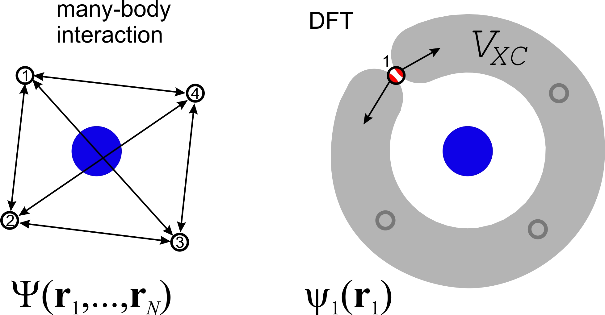
Figure shows many-body and DFT interactions schematically. Blue circles are nuclei and black hollow circles are electrons. In many-body approach, electrons have collective wave function ${\Psi}\left( {{{\bf{r}}_1},...,{{\bf{r}}_N}} \right)$ and interact between each other. In DFT approach, electron has individual wave function $\psi_1 \left( {\bf{r}}_1 \right)$ and interacts with $V_{XC}$ potential, which accounts many-body interactions. Red areas show schematically self-interaction.
Local Density Approximation
According to Hohenberg-Kohn theorem, the ground-state density uniquely determines the potential. This theorem allows us to consider DFT approach as exact substitute of many-body approach, if we know exact XC potential. However, we can calculate the XC potential only approximately.
The simplest way to approximate many-body interaction is the Local Density Approximation (LDA), when we treat electrons as the homogeneous electron gas and the exchange and correlation energies depend on electron density $\rho$. In Task 3 you will study direct formulas, how XC potential depends on $\rho$.
There are many different approaches to approximate many-body interaction between electrons more and more accurately, for example, Generalized Gradient Approximation (GGA) when energy depends not only on charge density but also on it's gradient too, or hybrid functionals, when the XC functional is the mix of two-electron Hartree-Fock potential with one-electron potential.
Self-interaction error
DFT approach, due to inaccuracy in accounting of many-body interaction in $V_{XC}$, leads to uncompensated interaction of electron with itself, unphysical electron self-interaction. As a consequence, this self-interaction error causes many problems, for example, significantly underpredicts chemical reaction barriers compared with experiments because of the tendency of DFT to overstabilize transition states with stretched bonds, the eigenvalue of the highest occupied KS orbital does not correspond to the ionization potential, as it should, underestimates band gap in semiconductors.
In order to correct self-interaction error, it was developed different self-interaction corrections (SIC), or you can use many-body approaches, like, for example, GW approximation, or Møller-Plesset (MP) approach.
Self-consistent field
Self-consistent field (SCF) method is used to solve KS equation numerically. We can start from some initial approximation to the solution. Let us suppose, that the set of $\psi_i^0$ and $\varepsilon_i^0$ is good initial guess to the solution. Using these values we can calculate KS potential and then solve KS equation with known potential. We will get new solution, $\psi_i^1$ and $\varepsilon_i^1$, from which we can recalculate new KS potential, $V^1$. Since using just new calculated potential $V^1$ can lead to divergence of iterations, we can set some mixing parameter $\alpha$ and calculate the potential for next iteration as following
- $$V^{NEW}={\alpha}V^1+\left(1-\alpha\right)V^0$$
where $0<\alpha \le 1$. In other words, we add only some part of the new calculated potential and keep part of the previous potential in order not to change the new solution, $\psi_i^1$ and $\varepsilon_i^1$, too much.
We can make several SCF iterations until we reach necessary accuracy for $\varepsilon_i$.
Software for DFT
There are available multiple DFT software with free or commercial license, written on different programming languages. These software may or may not use GPU accelerators. From physical point of view it can be written for different tasks and can use different basis set. For basis set it can use plane waves or Bloch sums for periodic systems like crystals, 2D materials, or polymers, or can use local basis functions, like Slater- or Gaussian-functions, which are more suitable to study separate molecules.
The list of available DFT software can be browsed on wiki page and in review article Compounds 2021, 1, 134.
In this course you will build your own DFT code from scratch.
Atomic units
In atomic units, more suitable for practical calculations, we set the charge of electron $e=1$, the mass of electron $m_e=1$, the Plank constant $\hbar=1$, and $4\pi {\varepsilon _0} = 1$. In this atomic units (a.u.), one a.u. of length is Bohr radius $a_0=$0.529177210903 $\unicode{x212B}$, and 1 a.u. of energy (1 Hartree) is 27.211386245988 $eV$.
Download Introduction as Word draft
Practical tasks
There are available two methods to practice in DFT coding:
- direct integration of the Kohn-Sham equation (level of difficulty 7/10);
- solving KS equation with the help of Green's functions (level of difficulty 10/10).
The task for both methods is the same
To calculate the lowest eigenvalue and eigenfunction of an isolated C5+ ion within the LDA using the Ceperley–Alder exchange–correlation functional as parameterized by Perdew and Zunger. Compare numerical solution with analytical solution from Schrödinger equation.
In order to solve this task we start from hydrogen-like atom (atom containing nucleus and one electron) and write analytical solution for lowest energy state. Then we consider such system from DFT point of view and solve Kohn-Sham equation numerically. In the end, you compare analytical solution with KS numerical solution.
In first method, direct integration of the Kohn-Sham equation, the global task is divided on 11 small tasks. The solutions are provided for tasks 1-10 with the programming modules on Fortran, C++, Python, and Julia.* Your task is to study these solutions and modules. In Task 11 you need to organize the SCF cycle to solve KS equation numerically by combining all studied modules, solve KS equation, and compare the analytical solution with the numerical solution.
There is also available short version of the course with level of difficulty 3/10, see Short course in the end of the page. In short version of the course you study two methods to solve differential equations numerically and study how to find solution of Schrödinger equation for H-like atom. After this short course you can convert the studied program to DFT level by adding $V^{XC}$ functional and organizing SCF cycle. The SCF cycle is necessary because $V^{XC}$ depends on the solution.
You can select any method to study or you can propose your own solution. If you just started study numerical methods it is highly recommended to start from the short course first.
You should make the solution well documented, because you can use it later for your PhD thesis.
In the end of the course you will be provided with the Certificate from Delta Science Institute and the recommendation on your LinkedIn page. In order to get the Certificate, you need to provide the solution for Method 1 or Method 2, or to provide your own method, the documentation of your solution including theoretical part, provide the developed programming module, the data files with the solution and graphs.
1 method. Direct integration of the radial Kohn-Sham equation
Task 1
Consider hydrogen-like atom in the ground state ($1s$). Write analytical expression for lowest eigenvalue and corresponding eigenfunction for hydrogen-like atom. Make programming module with this solution.
Tips: use Schrödinger equation in spherical coordinates and use symmetry condition for lowest energy state.
Literature: Pauling, L.; Wilson, E.B. Introduction to Quantum Mechanics, McGraw-Hill, New York, 1935
Task 2
Consider radial KS equation for H-like atom in $1s$ state.
Literature: Hartree, D.R. The calculation of atomic structures. Chapman & Hall, Ltd., London, 1957
Task 3
Make programming module for exchange-correlation potential $V^{XC}$.
Task 4
Write electron-electron repulsion potential for H-like atom using spherical symmetry.
Tips: use Poisson equation for charge density with boundary conditions.
Task 5
Study Numerov method to solve differential equation with boundary condition numerically.
Literature: Salvadori, M.G. Numerical methods in engineering. New York, 1952
Hint: In Numerov method, using finite differences you can transform differential equation to matrix equation. Since you have second derivative then the matrix will be tridiagonal. Next task describes the most efficient algorithm to solve tridiagonal matrix equation numerically.
Task 6
Study Thomas method to solve numerically tridiagonal matrix equation.
Hint: Thomas method is simplified method of Gaussian elimination. First sweep eliminates one element of matrix coefficients, and backward sweep produces solution. That's why this method also called double-sweep method.
Task 7
Develop numerical procedure to find e-e potential (Task 4) using Numerov (Task 5) and Thomas (Task 6) numerical methods.
Task 8
Develop numerical procedure to solve the radial KS equation with boundary conditions. Use Numerov and Thomas numerical algorithms.
Task 9
Develop the numerical procedure to calculate eigenvalue by integration KS equation.
Task 10
Write expression for total energy of the system in DFT approach (how $E_1$ depends on $\varepsilon_i$).
Literature: Parr, R.G.; Yang, W. Density functional theory of atoms and molecules. Oxford University Press, New York, 1989
Task 11
Organize SCF cycle to solve KS equation. Use analytical solution of Schrödinger equation as a starting point and use SCF mixing parameter $\alpha=0.1$ to find self-consistent solution. Plot the radial wavefunction calculated numerically and compare with analytical solution. Plot nucleus potential, e-e potential, XC potential. Find self-interaction error.
2 method. Solving KS equation with the help of Green functions
To use this method you need to be familiar with
- Complex analysis
- Residue theorem
- Green's function technique
In this exercise you will use the programming modules what you developed in first method: for XC and e-e potentials (Tasks 3 and 7), for eigenvalue (Task 9), and for total energy (Task 10).
Task 1
Write analytical expression for Green's function for the radial Schrödinger equation for H-like atom.
Task 2
Write the solution for KS equation for H-like atom using Green function from Task 1.
Task 3
Use residue theorem in order to find the solution from Task 2 numerically.
Task 4
Solve KS equation self-consistently by using exact analytical solution of Schrödinger equation as a starting point and use SCF mixing parameter $\alpha=0.1$. Play with $\alpha$ to understand convergence of SCF cycle.
Plot the radial wavefunction calculated numerically and compare with exact analytical solution.
Plot nucleus potential, e-e potential, XC potential. Find self-interaction error.
Basics of DFT
This is short version of the course without DFT programming. In this short course you will study two computational methods to solve differential equations, like Schrödinger equation, numerically.
Task 1
Study Introduction (download Introduction as Word draft). Answer the question, what is the difference between many-body and DFT approaches?
Task 2
Consider hydrogen-like atom in the ground state ($1s$). Use Schrödinger equation in spherical coordinates and write analytical expression for eigenvalue and eigenfunction for $1s$ state.
Literature: Pauling, L.; Wilson, E.B. Introduction to Quantum Mechanics, McGraw-Hill, New York, 1935
Task 3
Study Numerov method to solve differential equation with boundary condition numerically.
Literature: Salvadori, M.G. Numerical methods in engineering. New York, 1952
Hint: In Numerov method, using finite differences you can transform differential equation to matrix equation. Since you have second derivative then the matrix will be tridiagonal. Next task describes the most efficient algorithm to solve tridiagonal matrix equation numerically.
Task 4
Study Thomas method to solve tridiagonal matrix equation numerically.
Hint: Thomas method is simplified method of Gaussian elimination. First sweep eliminates one element of matrix coefficients, and backward sweep produces solution. That's why this method also called double-sweep method.
Task 5
Set eigenvalue to analytical solution from Task 2 and solve radial Schrödinger equation numerically using Numerov and Thomas algorithms. Plot numerical and analytical solutions for comparison.
Conclusion
In this course, you learned how a DFT program is organized — from setting up the SCF cycle to calculating the Hartree interaction and exchange–correlation potential.
You have seen how the Kohn–Sham equation is solved in practice and how the iterative mixing of potentials drives convergence.
This foundation gives you a clear understanding of how modern DFT codes operate at their core.
For those eager to continue, several add-ons are available — including relativistic extension, the use of external libraries for advanced XC functionals and for eigenvalue problem solver.
Keep exploring — the next step of DFT is just ahead!
* Please note, that the modules on C++, Python, and Julia were obtained from the original Fortran modules by line-by-line conversion with the help of ChatGPT (OpenAI)
© 2023-2026 Delta Science Institute
This course is freely available as an open educational resource.
Unless otherwise stated, the course materials are licensed under the
Creative Commons Attribution 4.0 International License (CC BY 4.0).
Preferred citation: Skachkov, D. (2026). Introduction to Density Functional Theory. Delta Science Institute. Available at: https://www.DSedu.org/courses/dft