Let us consider how to solve the Schrödinger equation if we know the eigenvalue.
We write the radial Schrödinger equation for $1s$ state (see Eq. (4) from Task 2) in the form:
- $$ - {1 \over 2} {d^2 \over{d{r^2}}} P\left( r \right) - \left( \varepsilon - V^{NUC}\left(r\right)\right) P\left(r\right) = 0$$
where $V^{NUC}$ is the nuclear potential
- $${V^{NUC}}\left( r \right) = - \frac{Z}{r}$$
and ${P}\left( r \right) = r{\Psi}\left( r \right)$ is the radial wave function,
Eq. (1) can be solved by Numerov method.
We will solve equation (1) on the region $\left[ {{r_0},{r_f}} \right]$, where r0 is a very small number and rf is sufficiently big number. We separate this region evenly by points $r_i, i=1,...,N$.
To simplify the task, we will set the values of the radial wave function at boundary points to analytical solution:
- $$\eqalign{
& P\left( r_0 \right) = P_{10}^0\left( r_0 \right) \cr
& P\left( r_f \right) = P_{10}^0\left( r_f \right) \cr} $$
where $P_{10}^0\left( r \right)$ is the analytical solution considered in Task 2 (see Eq. (6)).
Using Thomas method we look for solution in the form ${P_i} = {\alpha _{i + 1}}{P_{i + 1}} + {\beta _{i + 1}}$ (see Thomas method, formula (3)). As a first step, we find coefficients $\alpha_i$ and $\beta_i$ (see Thomas method, formula (4)), and for second step, calculate the solution $P_i$.
Using Eq. (3) for $P\left( {{r_0}} \right)$ we can define
- $$\eqalign{
& \alpha_2 = 0 \cr
& \beta_2 = P_{10}^0\left( r_0 \right)\cr} $$
Using Eqs. (4) from Thomas method we can calculate $\alpha_{i+1}$, $\beta_{i+1}$ for $i=2,...,N-1$.
For step two of Thomas method we calculate the functions $P_i$. For that, using Eq. (3) we set $P_N = P_{10}^0\left( r_f \right)$ and then using recurrent formula (3) from Thomas method, we can calculate
- $${P_i} = {\alpha _{i + 1}}{P_{i + 1}} + {\beta _{i + 1}}$$
for $i=N-1,...,2$, whereas $P_1$ is defined from Eq. (3).
Download the developed procedure in Fortran, C++, Python, or Julia module.
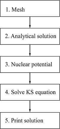
The block-diagram of the procedure:
Study the program and compile it.
If you use Fortran module, then use command:
ifx C_atom.f90 -o C_atom
If you use C++ module, then you can compile it with command:
g++ -O2 -std=c++11 C_atom.cpp -o C_atom
Then you can run the compiled module:
./C_atom
If you use Python, then run the program:
python C_atom.py
If you use Julia, then run the program:
julia C_atom.jl
These programs solve the Schrödinger equation for H-like atom and write the results into the file data.dat.
Use data file data.dat to plot the numerical solution ${P}\left( r \right)$ and check the error of calculation ${P}\left( r \right) - P_{10}^0\left( r \right)$.
Comments.
Change the boundary condition (3) to
$$\eqalign{
& P\left( r_0 \right) = 0 \cr
& P\left( r_f \right) = 0 \cr}$$
and check how the error of calculation is changing. Make $r_0$ smaller and $r_f$ larger to see how the solution will be closer to $P_{10}^0\left( r \right)$. Please note, that you can not set $r_0 = 0$ because of the nuclear potential (see Eq. (2)).