- Why is screening important?
- Polarization
- Screened Coulomb interaction
- The GW self-energy
- The connected GW equations
- Feynman-diagram representation of the GW equations
- Relation to Hedin’s equations
- From DFT to GW
- Common levels of GW calculations
- What GW describes
- What is not included in basic GW?
- Summary
- More advanced treatment
In the previous section, the self-energy $\Sigma$ was introduced as the quantity that modifies the reference Green’s function through the Dyson equation,
$$G^{-1} = G_0^{-1} - \Sigma.$$
The Dyson equation tells us how a known self-energy changes particle propagation. It does not, however, tell us how to calculate $\Sigma$.
The GW approximation provides a widely used approximation for the electronic self-energy:
$$\Sigma \approx iGW $$
Here, $G$ is the one-particle Green’s function and $W$ is the screened Coulomb interaction.
The name GW comes directly from this expression.
Why is screening important?
Two electrons interact through the Coulomb interaction.
The bare Coulomb interaction is denoted by $v$. It describes the interaction between two charges without accounting for the response of the surrounding material.
In a many-electron system, however, an electron polarizes the surrounding electron density. This induced polarization partially screens the original charge and modifies the interaction experienced by another electron.
The resulting effective interaction is called the screened Coulomb interaction $W$.
Thus,
$$v \quad\longrightarrow\quad W$$
represents the change from the bare interaction to the interaction modified by the electronic environment.
Polarization
The response of the electron system is described by the polarization $P$.
In the GW approximation, the polarization is written schematically as
$$P \approx -iGG $$
In the space-time representation, this expression takes the form
$$P(1,2)=-i\,G(1,2)G(2,1),$$
where $1\equiv(\mathbf r_1,t_1,\sigma_1)$ and $2\equiv(\mathbf r_2,t_2,\sigma_2)$ collectively denote the spatial, temporal, and spin coordinates.
More formally, an infinitesimal time shift $1^{+}$ may be introduced to ensure the correct time ordering and to avoid the ambiguity that arises in the Green’s function at equal times:
$$P(1,2)=-i\,G(1,2)G(2,1^{+})$$
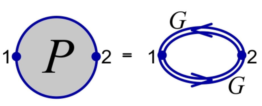
The two Green’s functions represent the propagation of an electron-hole pair created by the perturbing field.
Diagrammatically, this expression is represented by a closed bubble containing two fermionic propagator lines:
When the polarization is constructed without vertex corrections, the corresponding screening approximation is commonly associated with the random phase approximation.
The word “random” does not mean that the response is stochastic. It refers historically to the neglect of certain correlated phase relations between different particle-hole excitations.
In this approximation, screening is generated by independent particle-hole propagation.
Screened Coulomb interaction
The screened interaction satisfies
$$W = v + vPW $$
This equation has a simple physical interpretation.
The first term, $v$, is the bare Coulomb interaction.
The second term, $vPW$, describes an interaction modified by the polarization response of the surrounding electrons.
Substituting the equation for $W$ into itself gives
$$W = v + vPv + vPvPv + \cdots.$$
Thus, $W$ contains an infinite sequence of repeated polarization processes.
The screened interaction is therefore the bare Coulomb interaction dressed by the response of the electronic system.
The GW self-energy
Once the screened interaction has been constructed, the self-energy is approximated as
$$\Sigma \approx iGW$$
In the space-time representation, this expression becomes
$$\Sigma(1,2) = i\,G(1,2)\,W(2,1^{+}).$$
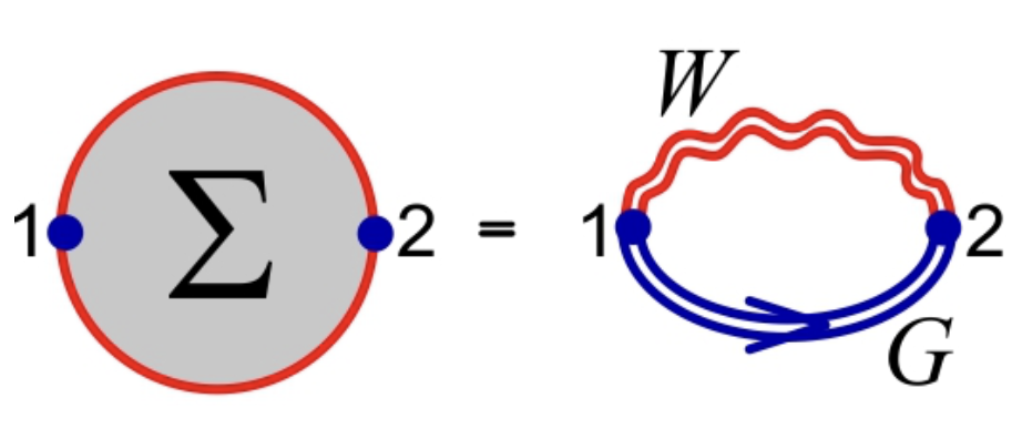
The Green’s function $G$ describes the propagation of the electron, while $W$ describes the screened interaction experienced during that propagation.
Diagrammatically, this expression is represented by a fermionic propagator line $G$ connected to a screened interaction line $W$:
When the self-energy acts on a Green’s function in the Dyson equation, it enters through the integral convolution
$$(\Sigma G)(1,2) = \int d3 \Sigma(1,3) G(3,2),$$
and therefore
$$(\Sigma G)(1,2) = i \int d3 G(1,3) W(1,3^{+}) G(3,2).$$
The screened interaction $W$ already contains the polarization response of the surrounding electrons through the relation
$$W=v+vPW.$$
Therefore, in the GW self-energy,
$$\Sigma=iGW,$$
the propagating electron described by $G$ interacts not only through the bare Coulomb interaction $v$, but also with the polarization that its electric field induces in the material. This induced polarization modifies the effective interaction experienced by the electron.
As a result, the self-energy changes the electron’s energy and gives the quasiparticle a finite lifetime, as discussed on the previous self-energy page.
The connected GW equations
The main quantities in the GW framework are related by four equations:
$$G = G_0 + G_0\Sigma G,$$
$$P = -iGG,$$
$$W = v + vPW,$$
$$\Sigma = iGW.$$
Starting from a Green’s function $G$:
- $G$ is used to calculate the polarization $P$;
- $P$ is used to construct the screened interaction $W$;
- $G$ and $W$ are used to calculate the self-energy $\Sigma$;
- $\Sigma$ is inserted into the Dyson equation to obtain an updated $G$.
This cycle may be evaluated once or repeated until self-consistency is reached.
In the space-time representation, the four equations of the GW approximation take the form
$$G(1,2) = G_0(1,2) + \int d3 d4 G_0(1,3) \Sigma(3,4) G(4,2) $$
$$P(1,2) = -i G(1,2) G(2,1^{+}) $$
$$W(1,2) = v(1,2) + \int d3 d4 v(1,3) P(3,4) W(4,2) $$
$$\Sigma(1,2) = i G(1,2) W(1^{+},2) $$
The products $G_0\Sigma G$ and $vPW$ are operator products and therefore become integral convolutions over intermediate space-time coordinates. By contrast, $P=-iGG$ and $\Sigma=iGW$ are direct products of two-point functions in the space-time representation.
The Dyson diagram for $G$ shows that the interacting propagator is obtained from the reference propagator by inserting the self-energy.
The polarization diagram contains two fermionic propagators forming a closed loop. It represents the electron-hole response of the system to a perturbation.
The screening diagram for $W$ shows that the screened interaction consists of the bare interaction v plus interaction processes modified by the polarization $P$.
Finally, the GW self-energy diagram combines one fermionic propagator $G$ with one screened interaction line $W$. This diagram is the origin of the name GW:
$$\Sigma = iGW.$$
Together, the four diagrams form the same closed cycle as the algebraic equations:
$$G \longrightarrow P \longrightarrow W \longrightarrow \Sigma \longrightarrow G.$$
The diagrammatic representation makes clear that the quantities are not calculated independently. Each one is constructed from the others, and the resulting system may be evaluated once or iterated until self-consistency is reached.
Feynman-diagram representation of the GW equations
The coupled GW equations can be represented graphically using the Feynman-diagram notation introduced earlier in this tutorial.
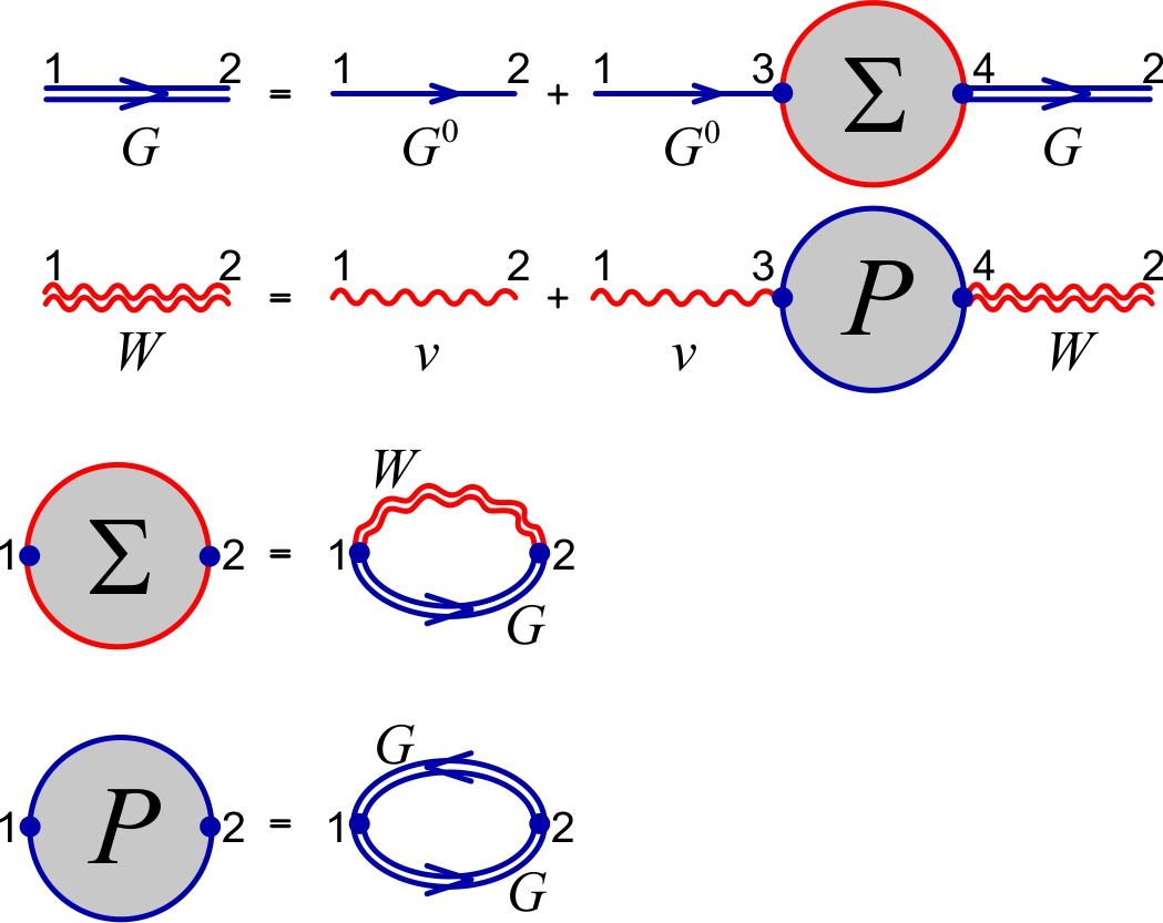
In the convention used in the figure:
- a thin solid line represents the reference Green’s function $G_0$;
- a double solid line represents the interacting Green’s function $G$;
- a single wavy line represents the bare Coulomb interaction $v$;
- a double wavy line represents the screened Coulomb interaction $W$;
- a polarization bubble represents $P$;
- a self-energy insertion represents $\Sigma$.
Relation to Hedin’s equations
The GW approximation is obtained from Hedin’s equations.
Hedin’s equations form an exact closed system for five quantities:
$$G, \qquad W, \qquad \Sigma, \qquad P, \qquad \Gamma,$$
where $\Gamma$ is the vertex function.
Schematically, the exact self-energy has the form
$$\Sigma = iGW\Gamma.$$
The exact polarization also depends on the vertex:
$$P = -iGG\Gamma.$$
In standard GW, the vertex is replaced by its simplest value:
$$\Gamma \approx 1.$$
This gives
$$\Sigma \approx iGW$$
and
$$P \approx -iGG.$$
Thus, the defining approximation of standard GW is not simply that it is a “first iteration.” More precisely, it is the approximation in which explicit vertex corrections are neglected.
After this approximation is made, the resulting GW equations may still be evaluated once or solved self-consistently.
From DFT to GW
In many practical calculations, the reference Green’s function $G_0$ is constructed from Kohn–Sham density functional theory.
Ground-state DFT is designed to reproduce the ground-state electron density. Its Kohn–Sham eigenvalues are not, in general, equal to the true charged excitation energies of the interacting system.
The GW self-energy is used to calculate quasiparticle corrections to these reference energies.
Schematically,
$$\text{DFT reference energies} \quad\longrightarrow\quad \text{GW quasiparticle energies}.$$
The exchange-correlation potential already included in the Kohn–Sham Hamiltonian must be removed when it is replaced by the GW self-energy.
A quasiparticle equation can be written as
$$E_{n\mathbf k}^{\mathrm{QP}} = \varepsilon_{n\mathbf k}^{\mathrm{KS}} + \left\langle n\mathbf k \left| \Sigma\!\left(E_{n\mathbf k}^{\mathrm{QP}}\right) - V_{\mathrm{xc}} \right| n\mathbf k \right\rangle.$$
Here, $\varepsilon_{n\mathbf k}^{\mathrm{KS}}$ is the Kohn–Sham energy, while $E_{n\mathbf k}^{\mathrm{QP}}$ is the corresponding quasiparticle energy.
Common levels of GW calculations
The coupled GW equations can be solved at different levels of self-consistency.
One-shot $G_0W_0$
In a $G_0W_0$ calculation, both the Green’s function and screened interaction are constructed from a fixed reference system, commonly DFT:
$$\Sigma \approx iG_0W_0. $$
The self-energy and quasiparticle corrections are then evaluated without fully updating the complete cycle.
This is the most widely used and computationally affordable form of GW.
Partially self-consistent GW
In partially self-consistent approaches, some quantities are updated while others remain fixed.
For example, quasiparticle energies may be updated in G, while the wave functions or screened interaction remain unchanged.
Self-consistent GW
In self-consistent GW, the quantities
$$G, \qquad P, \qquad W, \qquad \Sigma $$
are updated repeatedly until the calculation converges.
The resulting Green’s function is then consistent with the self-energy and screened interaction used to construct it.
What GW describes
The GW approximation is primarily used to calculate charged one-particle excitations, such as the energies required to add or remove an electron.
It is widely applied to:
- quasiparticle band structures;
- band gaps;
- ionization energies;
- electron affinities;
- band alignments;
- quasiparticle lifetimes;
- spectral properties.
Because screening is treated dynamically, GW often provides much better quasiparticle energies than the original Kohn–Sham eigenvalues.
What is not included in basic GW?
Standard GW uses
$$\Gamma \approx 1,$$
and therefore neglects explicit vertex corrections.
As a result, it does not contain every possible exchange-correlation process.
Electron-hole propagation contributes to the polarization $P$ and therefore to screening. However, the repeated attractive electron-hole interactions responsible for bound excitons are not included in a basic quasiparticle GW calculation.
Optical excitations and excitons are usually treated after GW by solving the Bethe–Salpeter equation.
Thus, the common workflow is
$$\text{DFT} \longrightarrow GW \longrightarrow \text{BSE}.$$
Here:
- DFT provides the reference electronic structure;
- GW provides quasiparticle energies;
- BSE describes interacting electron-hole excitations.
The approximation may also become less accurate when strong local correlations or large vertex corrections dominate. In such cases, methods beyond standard GW may be required.
Summary
The GW approximation provides an approximation for the self-energy:
$$\Sigma \approx iGW$$
The Green’s function $G$ describes electron propagation, while the screened interaction $W$ describes the Coulomb interaction modified by electronic polarization.
The central relations are
$$P = -iGG,$$
$$W = v+vPW,$$
$$\Sigma = iGW,$$
and
$$G = G_0+G_0\Sigma G.$$
Together, they describe the cycle
$$G \longrightarrow P \longrightarrow W \longrightarrow \Sigma \longrightarrow G.$$
More advanced treatment
For a more detailed discussion of Hedin’s equations, vertex corrections, diagrammatic expansions, frequency integrations, dielectric matrices, plasmon-pole models, self-screening, different levels of self-consistency, and practical GW implementations, see: More advanced topics in the GW approximation
Next: A Final Perspective